Principal Component Analysis (PCA) Explained

🧊 Principal Component Analysis (PCA)

PCA finds the most important directions in data and compresses the data into fewer numbers while trying to keep the important information

PCA is a dimensionality reduction algorithm that:

• finds directions of maximum variance
• projects data onto lower-dimensional space
• minimizes projection error

Run PCA only on the inputs to learn a mapping:

$$x \rightarrow z$$

where:

• $x \in \mathbb{R}^n$
• $z \in \mathbb{R}^k$
• $k \ll n$

Original training set:

$$(x^{(1)}, y^{(1)}), \dots, (x^{(m)}, y^{(m)})$$

Becomes:

$$(z^{(1)}, y^{(1)}), \dots, (z^{(m)}, y^{(m)})$$

Now the learning algorithm trains on lower-dimensional data.

Important:

• PCA map data of $n$ dimensions into $k$ dimensions
• PCA is an unsupervised algorithm
• PCA does not use labels $y$
• Do NOT fit PCA on:
  • cross-validation set
  • test set

The most widely used algorithm for dimensionality reduction.

Example:

Given a messy training data with

• 1000 features

PCA says:

“Maybe only 20 directions are really important.”

Advantages:

• Speed Up Learning: Lower-dimensional data makes training faster.
• Compression : Reduce storage and memory requirements.
• Visualization: visualization becomes easier for lower dimension

---

Bad Use of PCA

PCA is NOT a good method for preventing overfitting.

Some people think:

fewer dimensions = less overfitting

but this is not ideal.

Reason:

• PCA ignores labels $y$
• PCA may throw away useful predictive information

Instead:

✅ Use regularization to reduce overfitting.

Do NOT automatically add PCA to every ML pipeline.

Bad habit:

Training Data
    ↓
PCA
    ↓
Logistic Regression
    ↓
Predictions

Before using PCA, first try:

Training Data
    ↓
Learning Algorithm
    ↓
Predictions

Use PCA only if:

• training is too slow
• memory usage is too large
• dimensionality is extremely high

---

How to select $k$ in PCA?

A common way to choose the number of PCA components $k$ is by checking how much variance is retained.

PCA tries to minimize the projection error:

$$\frac{1}{m}\sum_{i=1}^{m} \left\|x^{(i)} - x^{(i)}_{approx}\right\|^2$$

where:

• $x^{(i)}$ = original data point
• $x^{(i)}_{approx}$ = projected/reconstructed point

The total variation in data is:

$$\frac{1}{m}\sum_{i=1}^{m} \left\|x^{(i)}\right\|^2$$

A standard rule is to choose the smallest $k$ such that:

$$\frac{ \frac{1}{m}\sum_{i=1}^{m} \left\|x^{(i)} - x^{(i)}_{approx}\right\|^2 }{ \frac{1}{m}\sum_{i=1}^{m} \left\|x^{(i)}\right\|^2 } \le 0.01$$

This means:

• projection error $\le 1\%$
• equivalently, 99% variance retained

People usually describe PCA quality as:

• 99% variance retained
• 95% variance retained
• 90% variance retained

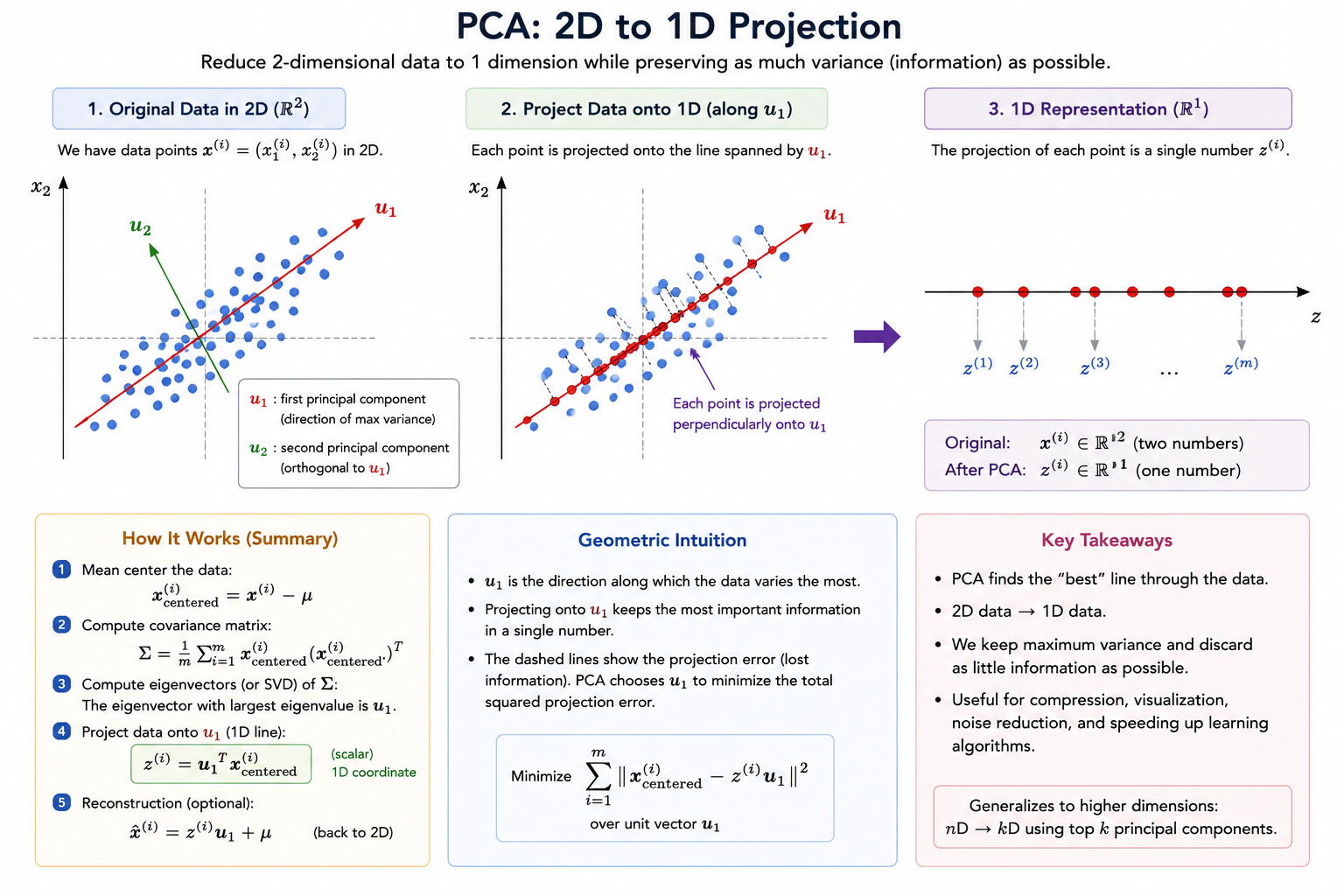
How to select Projection Direction?

A good projection line is one where:

• When we project each point onto the line
• The distance between the original point and its projection is small

⚠️ Projection errors

The orthogonal distance from a point to the line.

• Help with selecting projection direction

The projection error is:

$$\| x^{(i)} - \hat{x}^{(i)} \|^2$$

So goal of PCA is to find the direction that minimizes the total squared orthogonal distance.

$$\min_{u^{(1)}} \sum_{i=1}^{m} \| x^{(i)} - \text{projection of } x^{(i)} \text{ onto } u^{(1)} \|^2$$

where:

• $\hat{x}^{(i)}$ is the projected version of $x^{(i)}$

PCA minimizes:

$$\sum_{i=1}^{m} \| x^{(i)} - \hat{x}^{(i)} \|^2$$

Important:

• If PCA returns $u^{(1)}$ or $-u^{(1)}$, it does not matter.
• Both define the same line.

General Case: nD → kD

Now suppose:

$$x^{(i)} \in \mathbb{R}^n$$

Where $n$ is original number of dimensions

Example for 3D $n =3$

and we want to reduce to $k$ dimensions, eg. $k=2$ when we want to project 3D to 2D

$$z^{(i)} \in \mathbb{R}^k \quad \text{where } k < n$$

Instead of finding one vector, we find $k$ vectors:

$$u^{(1)}, u^{(2)}, \dots, u^{(k)}$$

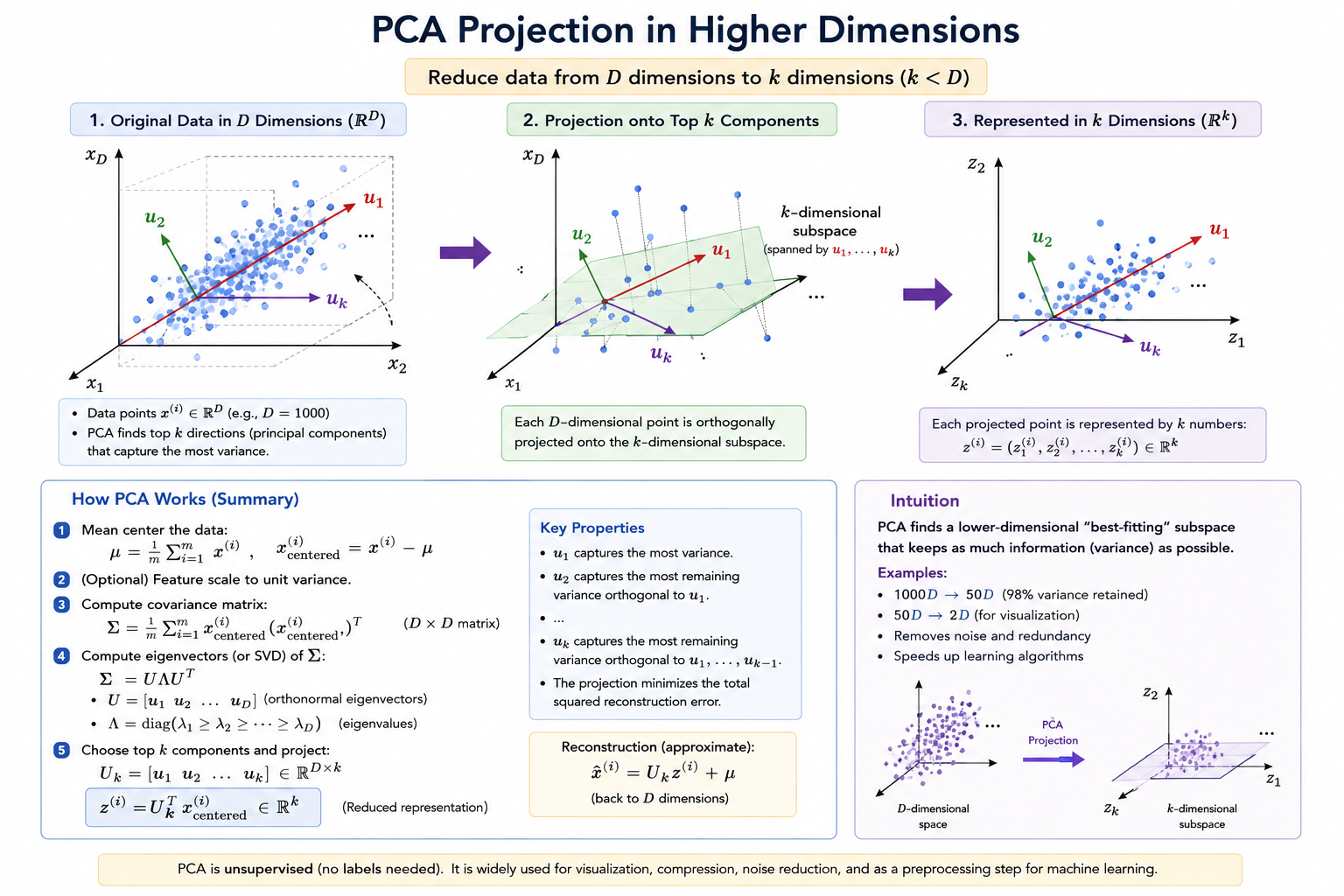
These vectors:

• Define a k-dimensional surface
• Span a k-dimensional linear subspace

We then project each point onto that subspace.

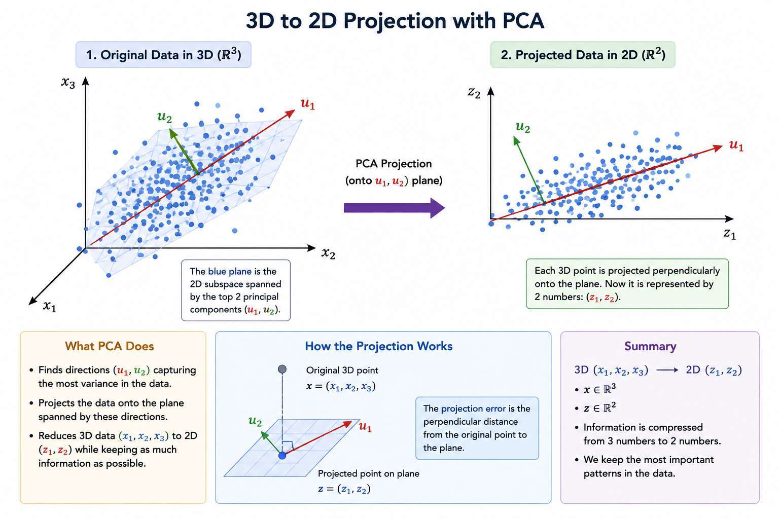
3D → 2D Example

If:

$$x^{(i)} \in \mathbb{R}^3$$

and we reduce to 2D:

• We find two vectors:

$$u^{(1)}, u^{(2)} \in \mathbb{R}^3$$

• These define a plane.
• Each point is projected onto that plane.

2D → 1D Example

Suppose we have:

$$x^{(i)} \in \mathbb{R}^2$$

and we want to reduce the data from 2 dimensions to 1 dimension.

That means:

• We want to find a line
• Onto which we project all data points

$$u^{(1)} \in \mathbb{R}^2$$

---

💡 PCA Algorithm

Suppose we have supervised learning data:

$$(x^{(i)}, y^{(i)})$$

where:

• $x^{(i)}$ = input features
• $y^{(i)}$ = labels

1. Ignore Labels Temporarily

Extract only the input vectors:

$x^{(1)}, x^{(2)}, x^{(3)}, x^{(4)}$

Before applying PCA, it is standard to:

1. Perform mean normalization

For each feature:

$$x_j := x_j - \mu_j$$

This makes each feature have zero mean.

2. Perform feature scaling (recommended)

Especially when features have different ranges.

$$x_j := \frac{x_j - \mu_j}{s_j}$$

where:

• $\mu_j$ = mean of feature $j$
• $s_j$ = standard deviation or feature range

So that:

• Each feature has zero mean
• Features have comparable ranges

This prevents one feature from dominating purely due to scale.

Step 2: Compute Covariance Matrix

Covariance Matrix ($\Sigma$)

is a square matrix giving the covariance between each pair of elements of a given random vector.

If:

• $m$ = number of examples
• $x^{(i)} \in \mathbb{R}^n$

then covariance matrix is:

$$\Sigma = \frac{1}{m}\sum_{i=1}^{m} x^{(i)}(x^{(i)})^T$$

Vectorized implementation:

$$\Sigma = \frac{1}{m}X^TX$$

import numpy as np

# Assuming data is (observations, features)
data = np.array([[1, 2, 3], [4, 5, 6], [7, 8, 9]])

# Set rowvar=False to treat columns as variables
cov_matrix = np.cov(data, rowvar=False) 

print(cov_matrix)

Step 3: Apply Singular Value Decomposition (SVD)

Compute Eugen Vector for Covariance Matrix ($\Sigma$)

$$[U,S,V] = SVD(\Sigma)$$

where

• $U$ is $nXn$ dimension matrix. $U = \begin{bmatrix}u_1 & u_2 & \dots & u_n\end{bmatrix}$

to take $k$ dimensions select first k columns

$U_{reduce} = \begin{bmatrix}u_1 & u_2 & \dots & u_k\end{bmatrix}$

• $S$ = diagonal matrix of singular values

$$S = \begin{bmatrix} S_{11} & 0 & 0 \\ 0 & S_{22} & 0 \\ 0 & 0 & \ddots \end{bmatrix}$$

Then variance retained can be computed efficiently as:

$$\frac{ \sum_{i=1}^{k} S_{ii} }{ \sum_{i=1}^{n} S_{ii} }$$

Choose the smallest $k$ such that:

$$\frac{ \sum_{i=1}^{k} S_{ii} }{ \sum_{i=1}^{n} S_{ii} } \ge 0.99$$

for 99% variance retained.

Typical values:

• 90%
• 95%
• 99%

Most commonly:

• 95% to 99% variance retained.

• $V$ = right singular vectors (not used in PCA)

import numpy as np

# Define your matrix
A = np.array([[1, 2], [3, 4], [5, 6]])

# Perform SVD
U, S, Vt = np.linalg.svd(A)

print("U (Left Singular Vectors):\n", U)
print("\nS (Singular Values as 1D array):\n", S)
print("\nVt (Right Singular Vectors - Transposed):\n", Vt)

Step 4: Choose Top K Components

Take the first $k$ columns:

$$U_{reduce} = [u_1 \ u_2 \ ... \ u_k]$$

This reduces data from:

• $n$ dimensions to
• $k$ dimensions

Step 5: Project Data

Compute reduced representation:

$$z = U_{reduce}^T x$$

Which is equivalent to

$$z_j = (u^{(j)})^{T}x$$

where:

• $x \in \mathbb{R}^n$ : represents the original input values in n dimension
• $z \in \mathbb{R}^k$ : represents the coordinates of $x$ in the reduced k-dimensional space.
• $U_{reduce}^T = \begin{bmatrix}u_1^T \\ u_2^T \\ \vdots \\ u_k^T\end{bmatrix}$

---

Reproduce $x_i$ from given $z$

We know

$$z = U_{reduce}^T x$$

we can calculate $x$

$$x_{approx} = z U_{reduce}$$

Where

• $z$ is $k X 1$ matrix
• $U_{reduce}$ is $n X k$ matrix

---

PCA vs Linear Regression (Very Important)

PCA is NOT linear regression.

Linear Regression:

• Predicts a special variable $y$
• Minimizes vertical squared errors
• Error is measured in the y-direction only

PCA:

• Has no special target variable
• All features $x_1, x_2, \dots, x_n$ are treated equally
• Minimizes orthogonal (shortest) distance to a line/plane

Linear regression minimizes:

$$\text{vertical distance}$$

PCA minimizes:

$$\text{orthogonal distance}$$

These are completely different objectives.

---

Final Summary

PCA:

• Finds a lower-dimensional subspace
• Projects data onto that subspace
• Minimizes squared orthogonal projection error
• Treats all features symmetrically
• Is not a predictive model

Formally, PCA solves:

$$\min \sum_{i=1}^{m} \| x^{(i)} - \hat{x}^{(i)} \|^2$$

where $\hat{x}^{(i)}$ is the projection of $x^{(i)}$ onto a k-dimensional subspace.

---