
Data Structures & Algorithms (DSA) & Database Management System (DBMS)
🧱 Data Structures
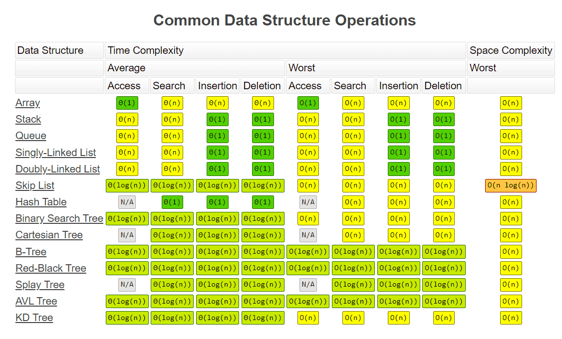
Linear Data Structures
| # | Data Structure | Access | Insertion | Deletion | Searching |
|---|---|---|---|---|---|
| 1️⃣ | 🧮 Array | ⚡ O(1) | ⏳ At 0 Index: O(n) | ⏳ At 0 Index: O(n) | 🔍 Linear: O(n)Binary (Sorted): O(log n) |
| 2️⃣ | 🔗 Linked List | ⏳ O(n) | ⚡ O(1) | ⚡ O(1) | 🔍 O(n) |
| 3️⃣ | 📚 Stack | ⏳ O(n) | ⚡ O(1) | ⚡ O(1) | 🔍 O(n) |
| 4️⃣ | 🚶 Queue | ⏳ O(n) | ⚡ O(1) | ⚡ O(1) | 🔍 O(n) |
🌲 Non-Linear Data Structures
| # | Data Structure | Access | Insertion | Deletion | Searching | Space |
|---|---|---|---|---|---|---|
| 1️⃣ | 🌿 AVL Tree | ⚡ O(log n) | ⚡ O(log n) | ⚡ O(log n) | ⚡ O(log n) | 💾 O(n) |
| 2️⃣ | 🌳 Binary Search Tree (BST) | 🐢 O(n) | 🐢 O(n) | 🐢 O(n) | 🐢 O(n) | 💾 O(n) |
| 3️⃣ | 🌴 B-Tree | ⚡ O(log n) | ⚡ O(log n) | ⚡ O(log n) | ⚡ O(log n) | 💾 O(n) |
| 4️⃣ | 📐 Cartesian Tree | N/A | ⏳ O(n) | ⏳ O(n) | ⏳ O(n) | 💾 O(n) |
| 5️⃣ | 📊 KD Tree | ⚡ O(log n) | ⚡ O(log n) | ⚡ O(log n) | ⚡ O(log n) | 💾 O(n) |
| 6️⃣ | 🔴 Red-Black Tree | ⚡ O(log n) | ⚡ O(log n) | ⚡ O(log n) | ⚡ O(log n) | 💾 O(n) |
| 7️⃣ | 🪜 Skip List / Skip Tree | ⚡ O(log n) | ⚡ O(log n) | ⚡ O(log n) | ⚡ O(log n) | 💾 O(n) |
| 8️⃣ | 🌀 Splay Tree | ⚖️ Amortized O(log n) | ⚖️ Amortized O(log n) | ⚖️ Amortized O(log n) | ⚖️ Amortized O(log n) | 💾 O(n) |
| 9️⃣ | ⛰️ Binary Heap | ⏳ O(log n) | ⚡ O(log n) | ⏳ O(log n) | 🔍 O(n) | 💾 O(n) |
| 🔟 | 🧩 Hash Table | ❌ N/A | ⚡ O(1) | ⚡ O(1) | ⚡ O(1) | 💾 O(n) |
Note:
H = log n for self-balancing BSTs such as AVL, Red-Black, and Splay Trees — they maintain a logarithmic height.
🧠 Other Advanced Structures
| # | Data Structure | Access | Insertion | Deletion | Searching | Space |
|---|---|---|---|---|---|---|
| 1️⃣ | 🕸️ Graph | O(1) (Adj. Matrix)O(V + E) (Adj. List) | ⚡ O(1) | ⏳ O(V + E) | 🔍 O(V + E) | 💾 O(V + E) |
| 2️⃣ | 🔤 Trie | ⏳ O(L) | ⏳ O(L) | ⏳ O(L) | ⏳ O(L) | 💾 O(ALPHABET_SIZE × n) |
| 3️⃣ | 📏 Segment Tree | ⚡ O(log n) | ⚡ O(log n) | ⚡ O(log n) | ⚡ O(log n) | 💾 O(n) |
| 4️⃣ | 🧬 Suffix Tree | ⚡ O(n) | ⚡ O(n) | ⚡ O(n) | ⚡ O(m) | 💾 O(n) |
📈 Asymptotic Notations / Landau Notation (Edmund Landau)
Measures the order of growth of an algorithm with respect to the number of inputs n.
Big O
Represents the worst-case scenario, where the loop runs till the last element.
- Simplified Worst case when loop runs till the last elements:
- Fastest growing expression determine over all complexity.
- Remove Constant & Remove non-dominant terms
Example.
f(n) = An+B
= O(n)

f(n) = n3+n2+7n
= O(n3)
Common used big O notation
| Complexity | Visual Growth | Description |
|---|---|---|
| O(1) | 🟢 | Constant — fastest, independent of n |
| O(log n) | 🟢🟢 | Logarithmic — grows slowly, e.g., Binary Search |
| O(n) | 🟡🟡🟡 | Linear — grows proportionally to input size |
| O(n log n) | 🟡🟡🟡🟡 | Polylogarithmic — e.g., Merge Sort, Quick Sort (average) |
| O(n²) | 🔴🔴🔴🔴 | Quadratic — nested loops, e.g., Bubble Sort |
| O(n³) | 🔴🔴🔴🔴🔴 | Cubic — triple nested loops |
| O(cⁿ) | 🔴🔥 | Exponential — runtime doubles/triples with each input |
| O(n!) | 🔥🔥🔥 | Factorial — extremely fast growth, e.g., brute-force permutations |
🟢 1. Optimized (Lower Growth Order)
O(1) - Constant time
- Single R/W
- Single statement of code
- No loops
- A loop which run in fix number of time
O(log(n)) - Logarithmic
- Loop divided by constant number eg Binary Serach
- Divide & conqure
O(n(log(n)) - PolyLogarithmic
- Loop divided & multiplied by constant number
🔴 2. Not Optimized (Higher Growth Order)
| Complexity | Type | Description |
|---|---|---|
| O(n) | Linear | Loop increases/decreases by constant number |
| O(nᶜ) | Polynomial | C nested loops |
| O(n²) | Quadratic | 2 nested loops |
| O(n³) | Cubic | 3 nested loops |
| O(cⁿ) | Exponential | For each element run C nested loops |
| O(n!) | Factorial | Adds a loop for every element |
Notes:
- O(cⁿ) grow faster than O(nᶜ). If O(nᶜ) grow faster than O(cⁿ) than it is called superpolynomial & in that case O( cⁿ) called subexponential
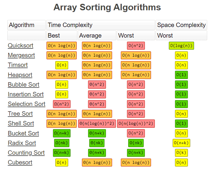
⚡ Sorting Algorithm Complexity
Legend
- Ω (Omega) → Best case
- Θ (Theta) → Average case
- O (Big O) → Worst case
- Stable? ✅ Yes / ❌ No
| # | Algorithm | ⏱️ Best | ⚖️ Average | 🔻 Worst | 💾 Space | ⚙️ Stability |
|---|---|---|---|---|---|---|
| 1️⃣ | ⚡ Quick Sort | Ω(n log n) | Θ(n log n) | O(n²) | O(log n) | ❌ No |
| 2️⃣ | 🧩 Merge Sort | Ω(n log n) | Θ(n log n) | O(n log n) | O(n) | ✅ Yes |
| 3️⃣ | 🚀 Timsort | Ω(n) | Θ(n log n) | O(n log n) | O(n) | ✅ Yes |
| 4️⃣ | ⛰️ Heap Sort | Ω(n log n) | Θ(n log n) | O(n log n) | O(1) | ❌ No |
| 5️⃣ | 💧 Bubble Sort | Ω(n) | Θ(n²) | O(n²) | O(1) | ✅ Yes |
| 6️⃣ | ✍️ Insertion Sort | Ω(n) | Θ(n²) | O(n²) | O(1) | ✅ Yes |
| 7️⃣ | 🪞 Selection Sort | Ω(n²) | Θ(n²) | O(n²) | O(1) | ❌ No |
| 8️⃣ | 🌲 Tree Sort | Ω(n log n) | Θ(n log n) | O(n²) | O(n) | ✅ Yes |
| 9️⃣ | 🐚 Shell Sort | Ω(n log n) | Θ(n (log n)²) | O(n (log n)²) | O(1) | ❌ No |
| 🔟 | 🪣 Bucket Sort | Ω(n + k) | Θ(n + k) | O(n²) | O(n) | ✅ Yes |
| 1️⃣1️⃣ | 🔢 Radix Sort | Ω(n k) | Θ(n k) | O(n k) | O(n + k) | ✅ Yes |
| 1️⃣2️⃣ | 🧮 Counting Sort | Ω(n + k) | Θ(n + k) | O(n + k) | O(k) | ✅ Yes |
| 1️⃣3️⃣ | 🧊 Cube Sort | Ω(n) | Θ(n log n) | O(n log n) | O(n) | ✅ Yes |
🔎 Searching Algorithm Complexity
| # | Algorithm | ⏱️ Best | ⚖️ Average | 🔻 Worst | 💾 Space | ⚙️ Stability |
|---|---|---|---|---|---|---|
| 1️⃣ | 🚶♂️ Linear Search | O(1) | O(n) | O(n) | O(1) | ✅ Yes |
| 2️⃣ | 🎯 Binary Search | O(1) | O(log n) | O(log n) | O(1) | ✅ Yes |
| 3️⃣ | 🪜 Jump Search | O(1) | O(√n) | O(√n) | O(1) | ✅ Yes |
| 4️⃣ | 🧩 Interpolation Search | O(1) | O(log log n) | O(n) | O(1) | ✅ Yes |
| 5️⃣ | ⚡ Exponential Search | O(1) | O(log n) | O(log n) | O(1) | ✅ Yes |
| 6️⃣ | 🧮 Fibonacci Search | O(1) | O(log n) | O(log n) | O(1) | ✅ Yes |
| 7️⃣ | 🔢 Hashing Search | O(1) | O(1) | O(n) | O(n) | ✅ Yes |
| 8️⃣ | 🌳 Binary Search Tree (BST) | O(1) | O(log n) | O(n) | O(n) | ✅ Yes |
| 9️⃣ | 🌲 Balanced BST (AVL, Red-Black) | O(1) | O(log n) | O(log n) | O(n) | ✅ Yes |
Notes
- Binary Search requires sorted data.
- Hashing gives average constant-time lookup but degrades to O(n) on collisions.
- Balanced Trees ensure logarithmic performance by maintaining structure.
- Jump and Interpolation searches are useful for uniformly distributed data.
🗄️ Database Comparison
| DB | Paradigm | Key Features | Use Case / Space / Notes |
|---|---|---|---|
| Redis | 🔑 Key-Value | In-Memory, PUB/SUB, Caching | Leaderboards, Session Storage 🟢 |
| Cassandra | 🟩 Wide Column | Schema-less, No Joins | High write throughput, Time Series ⏱️ |
| HBase | 🟩 Wide Column | Schema-less, No Joins | Large-scale storage, Batch Processing 🟡 |
| MongoDB / Firebase / CouchDB / Dynamo | 📄 Document-Oriented | Schema-less, No Joins | IOT, Games, Fast Reads & Writes 🎮 |
| MySQL (Oracle) / PostgreSQL | 🗂️ Relational | Schema, Join, ACID | Banking, Enterprise Applications 🏦 |
| Neo4J | 🌐 Graph | Relationships, Graph Queries | Knowledge Graphs, Recommendations 🌐 |
| Solr / Algolia / Elasticsearch | 🔎 Search Index | Indexing, Full-text Search | Search Engines 🔍 |
| Fauna / GraphQL | ⚡ Multi-Model | Flexible, Multi-paradigm | Modern APIs, Not restricted to one model ⚡ |