🌲 Trees Deep Dive: BST, AVL Rotations, Red-Black Trees, B-Trees & B+ Trees
The tree family from the ground up — Binary Tree and BST fundamentals, DFS/BFS traversal, why an unbalanced BST degrades to O(n), all four AVL rotation cases worked through step by step, Red-Black Tree's five properties with search and insert, B-Trees and B+ Trees for database indexing, plus hash tables and tries.
🧱 Data Structures: Arrays, Stacks, Queues, Heaps, Hash Tables, Tries & Graphs
🕸️ Graph Data Structures: Adjacency List vs Matrix, BFS & DFS
Non-Linear Data Structures
In a linear structure each element has a single successor — you walk it end to end.
A non-linear structure is hierarchical (trees) or networked (graphs): one element connects to many, so there's no single "next."
That branching is exactly what buys the operations below — and every one of those logs quietly assumes something (balance, a good hash, the right representation). The table states the headline; the sections below state the assumption.
    Non-Linear Data Structures
    │
    ├── Trees
    │   ├── Tree Fundamentals
    │   ├── Binary Tree
    │   ├── Binary Search Tree
    │   ├── AVL Tree
    │   ├── Red-Black Tree
    │   ├── B-Tree
    │   ├── B+ Tree
    │   └── Heap
    │
    ├── Trie
    │
    ├── Hash Table
    │
    └── Graphs
        ├── Graph Representation
        ├── BFS
        ├── DFS
        ├── Shortest Path
        ├── Minimum Spanning Tree
        └── Topological Sort
| # | Structure | Search 🔍 | Insert ➕ | Delete 🗑️ | Space |
|---|---|---|---|---|---|
| 1 | 🌳 BST (unbalanced) | avg : worst: | Avg: Worst: | Avg: Worst: | |
| 2 | ⚖️ Balanced BST (AVL/RB) | ||||
| 3 | ⛰️ Binary Heap | peek: | (extract root) | ||
| 4 | #️⃣ Hash Table | Avg Worst: | Avg: Worst: | Avg: Worst: | |
| 5 | 🔤 Trie | ||||
| 6 | 🕸️ Graph | see representation below | edge: – | edge: – | List: Matrix: |
Broader Tree Family
| # | Data Structure | Access | Insertion | Deletion | Searching | 💾 Space |
|---|---|---|---|---|---|---|
| 1 | 🌳 Binary Search Tree (BST) | |||||
| 2 | 🌿 AVL Tree | |||||
| 3 | 🔴 Red-Black Tree | |||||
| 4 | 🌴 B-Tree | |||||
| 5 | 📐 Cartesian Tree | N/A | ||||
| 6 | 📊 KD Tree | |||||
| 7 | 🪜 Skip List / Skip Tree | |||||
| 8 | 🌀 Splay Tree | Amortized | Amortized | Amortized | Amortized |
Note:
for self-balancing BSTs such as AVL, Red-Black, and Splay Trees — they maintain a logarithmic height.
TREE Data Structure
A tree is a hierarchical data structure consisting of
nodesconnected byedges.
Tree is the fundamental building block for Tree base advance Data structure.
Unlike linear data structures, each node can have multiple children, forming a parent-child hierarchy.
flowchart TB
    A["Root 🌳"]
    A --> B["Parent"]
    A --> C["Parent"]
    A --> D["Parent"]

    B --> E["Leaf 🍃"]
    B --> F["Leaf 🍃"]
    C --> G["Leaf 🍃"]

    D --> H["Leaf 🍃"]
    D --> I["Leaf 🍃"]
Node Properties
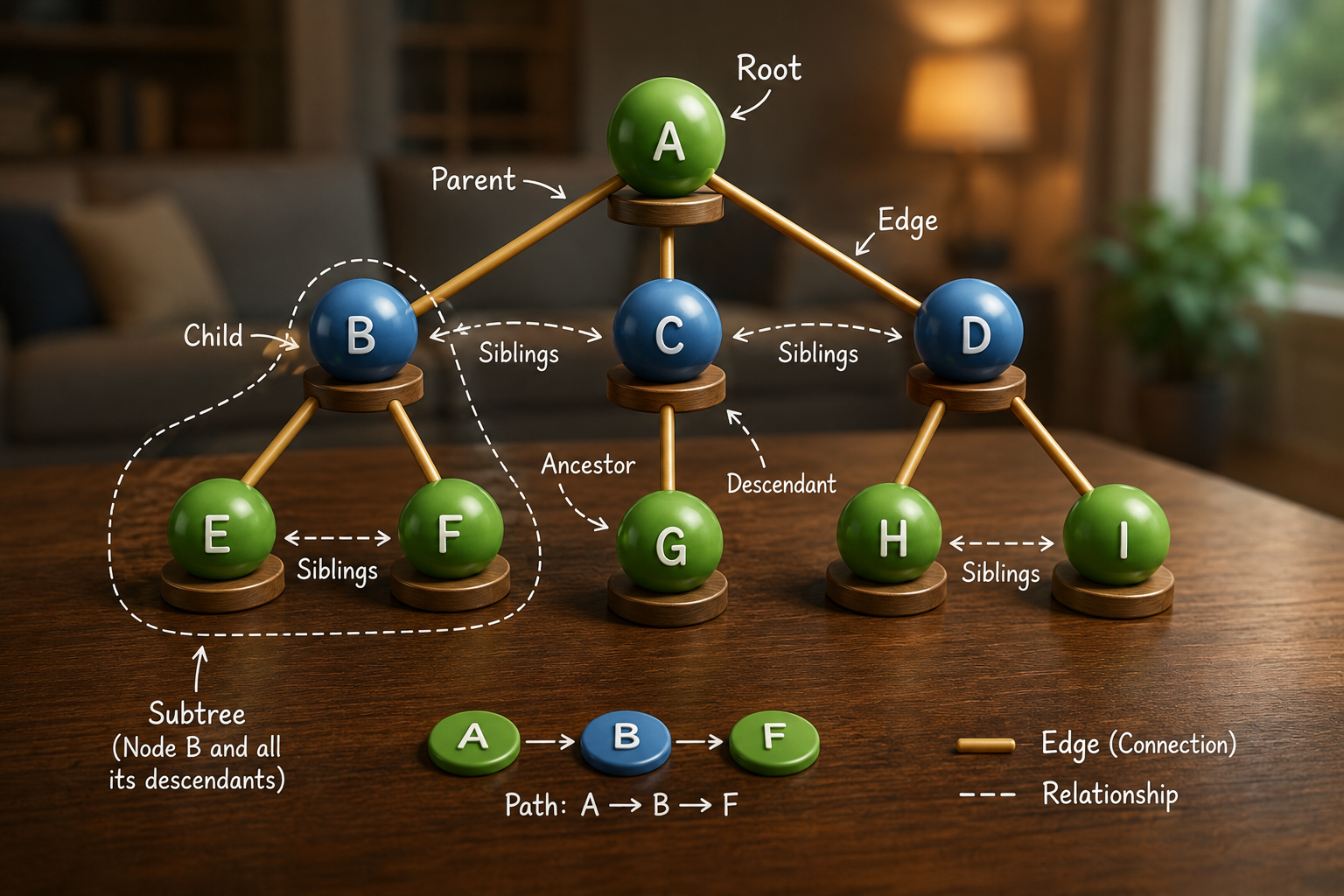
| Property | Description | |
|---|---|---|
| 🌳 | Root | The top-most node of the tree. It has no parent. |
| 👨👧 | Parent | A node that directly connects to one or more child nodes. |
| 🔗 | Edge | A connection between a parent and a child node. |
| 🛤️ | Path | A sequence of nodes connected by edges. |
| 👶 | Child | A node directly connected below a parent. |
| 🌿 | Internal Node | A node with at least one child. |
| 🍃 | Leaf | A node with no children. Also called an external node. |
| 👨👩👧 | Sibling | Nodes that share the same parent. |
| 🌲 | Ancestor | Any node on the path from the root to a given node. |
| 🌾 | Descendant | Any node reachable by repeatedly following child links from a node. |
| 🌱 | Subtree | A tree formed by a node and all of its descendants. |
Tree Dimensions
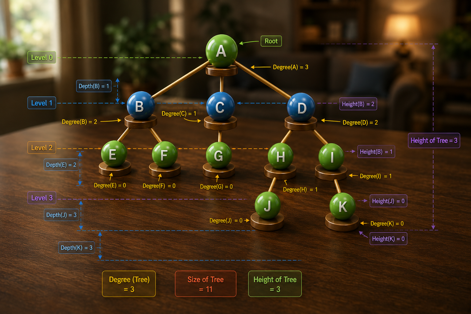
| Property | Description | |
|---|---|---|
| Property | Description | |
| 📏 | Depth | The number of edges from the root to a node. |
| 📐 | Height | The number of edges on the longest path from a node to a leaf. |
| 📊 | Height of Tree | The height of the root node, representing the maximum depth of the tree. |
| 📚 | Level | The position of a node in the tree. The root is typically at Level 0 (or Level 1 by some conventions). |
| 🌟 | Degree (Node) | The number of children a node has. |
| 🌍 | Degree (Tree) | The maximum degree of any node in the tree. |
| 📦 | Size | The total number of nodes in the tree. |
Node have value and pointer to its child
class TreeNode {
  constructor(value) {
    this.value = value;
    this.children = [];
  }

  addChild(node) {
    this.children.push(node);
  }
}
✅ Advantages
- Naturally represents hierarchical data
- Supports multiple children
- Flexible structure
- Easy recursive algorithms
❌ Limitations
- Slower search than hash tables
- No inherent ordering
- Traversal often required
Tree Properties
| Operation | Time Complexity | Reason |
|---|---|---|
| 🔍 Search | May need to visit every node. | |
| ➕ Insert | * | If the parent node is already known. |
| ➕ Insert | If the parent must first be searched. | |
| 🗑️ Delete | Must locate the node before removing it. | |
| 🔄 Traversal | Every node is visited exactly once. |
Note: These complexities are for a general (non-search) tree. Since nodes are not ordered, operations such as search and delete may require traversing the entire tree.
BINARY TREE DataStructure (BT)
A Binary Tree is a tree in which each node has at most two children, commonly referred to as the left child and right child.
Unlike a Binary Search Tree (BST), a binary tree does not enforce any ordering between node values.
flowchart TB
  N50(("50"))

  N50 --> N30(("30"))
  N50 --> N70(("70"))

  N30 --> N20(("20"))
  N30 --> N40(("40"))

  N70 --> N60(("60"))
  N70 --> N80(("80"))

%% Extra nodes
  N40 --> N35(("35"))
  N40 --> N45(("45"))

  N80 --> N90(("90"))

%% Root
  style N50 fill:#10B981,stroke:#047857,stroke-width:3px,color:#ffffff

%% Internal Nodes
  style N30 fill:#3B82F6,stroke:#1D4ED8,stroke-width:2px,color:#ffffff
  style N70 fill:#3B82F6,stroke:#1D4ED8,stroke-width:2px,color:#ffffff
  style N40 fill:#3B82F6,stroke:#1D4ED8,stroke-width:2px,color:#ffffff
  style N80 fill:#3B82F6,stroke:#1D4ED8,stroke-width:2px,color:#ffffff

%% Leaf Nodes
  style N20 fill:#F59E0B,stroke:#B45309,stroke-width:2px,color:#ffffff
  style N60 fill:#F59E0B,stroke:#B45309,stroke-width:2px,color:#ffffff
  style N35 fill:#F59E0B,stroke:#B45309,stroke-width:2px,color:#ffffff
  style N45 fill:#F59E0B,stroke:#B45309,stroke-width:2px,color:#ffffff
  style N90 fill:#F59E0B,stroke:#B45309,stroke-width:2px,color:#ffffff

%% Edge styling
  linkStyle default stroke:#64748B,stroke-width:2px
Binary Tree Properties
-
Each node has 0, 1, or 2 children
-
Every child is either a left child or right child
-
No ordering exists between parent and children
-
Height depends on the tree's shape
-
Traversals include Preorder, Inorder, Postorder, and Level Order
1. Full Binary Tree
Every node has either 0 or 2 children.
- Every internal node has exactly two children.
- All leaf nodes are at the same level.
flowchart TB
    N50(("50"))

    N50 --> N30(("30"))
    N50 --> N70(("70"))

    N30 --> N20(("20"))
    N30 --> N40(("40"))

    N70 --> N60(("60"))
    N70 --> N80(("80"))

    %% Left subtree
    N40 --> N35(("35"))
    N40 --> N45(("45"))

    %% Right subtree
    N80 --> N75(("75"))
    N80 --> N90(("90"))

    %% Root
    style N50 fill:#10B981,stroke:#047857,stroke-width:3px,color:#ffffff

    %% Internal Nodes
    style N30 fill:#3B82F6,stroke:#1D4ED8,stroke-width:2px,color:#ffffff
    style N70 fill:#3B82F6,stroke:#1D4ED8,stroke-width:2px,color:#ffffff
    style N40 fill:#3B82F6,stroke:#1D4ED8,stroke-width:2px,color:#ffffff
    style N80 fill:#3B82F6,stroke:#1D4ED8,stroke-width:2px,color:#ffffff

    %% Leaf Nodes
    style N20 fill:#F59E0B,stroke:#B45309,stroke-width:2px,color:#ffffff
    style N35 fill:#F59E0B,stroke:#B45309,stroke-width:2px,color:#ffffff
    style N45 fill:#F59E0B,stroke:#B45309,stroke-width:2px,color:#ffffff
    style N60 fill:#F59E0B,stroke:#B45309,stroke-width:2px,color:#ffffff
    style N75 fill:#F59E0B,stroke:#B45309,stroke-width:2px,color:#ffffff
    style N90 fill:#F59E0B,stroke:#B45309,stroke-width:2px,color:#ffffff

    linkStyle default stroke:#64748B,stroke-width:2px
2. Perfect Binary Tree
All internal nodes have two children, and all leaves are at the same level.
flowchart TB
    N50(("50"))

    N50 --> N30(("30"))
    N50 --> N70(("70"))

    N30 --> N20(("20"))
    N30 --> N40(("40"))

    N70 --> N60(("60"))
    N70 --> N80(("80"))

    N20 --> N10(("10"))
    N20 --> N25(("25"))

    N40 --> N35(("35"))
    N40 --> N45(("45"))

    N60 --> N55(("55"))
    N60 --> N65(("65"))

    N80 --> N75(("75"))
    N80 --> N90(("90"))

    %% Root
    style N50 fill:#10B981,stroke:#047857,stroke-width:3px,color:#fff

    %% Internal Nodes
    style N30 fill:#3B82F6,stroke:#1D4ED8,stroke-width:2px,color:#fff
    style N70 fill:#3B82F6,stroke:#1D4ED8,stroke-width:2px,color:#fff
    style N20 fill:#3B82F6,stroke:#1D4ED8,stroke-width:2px,color:#fff
    style N40 fill:#3B82F6,stroke:#1D4ED8,stroke-width:2px,color:#fff
    style N60 fill:#3B82F6,stroke:#1D4ED8,stroke-width:2px,color:#fff
    style N80 fill:#3B82F6,stroke:#1D4ED8,stroke-width:2px,color:#fff

    %% Leaf Nodes
    style N10 fill:#F59E0B,stroke:#B45309,stroke-width:2px,color:#fff
    style N25 fill:#F59E0B,stroke:#B45309,stroke-width:2px,color:#fff
    style N35 fill:#F59E0B,stroke:#B45309,stroke-width:2px,color:#fff
    style N45 fill:#F59E0B,stroke:#B45309,stroke-width:2px,color:#fff
    style N55 fill:#F59E0B,stroke:#B45309,stroke-width:2px,color:#fff
    style N65 fill:#F59E0B,stroke:#B45309,stroke-width:2px,color:#fff
    style N75 fill:#F59E0B,stroke:#B45309,stroke-width:2px,color:#fff
    style N90 fill:#F59E0B,stroke:#B45309,stroke-width:2px,color:#fff

    linkStyle default stroke:#64748B,stroke-width:2px
3. Complete Binary Tree
Every level is completely filled except possibly the last, which is filled from left to right.
- Every level is completely filled except possibly the last.
- The last level is filled from left to right without gaps.
Unlike a Perfect Binary Tree, the last level does not have to be full.
- Used by Binary Heaps.
flowchart TB
    N50(("50"))

    N50 --> N30(("30"))
    N50 --> N70(("70"))

    N30 --> N20(("20"))
    N30 --> N40(("40"))

    N70 --> N60(("60"))
    N70 --> N80(("80"))

    N20 --> N10(("10"))
    N20 --> N25(("25"))

    N40 --> N35(("35"))

    %% Root
    style N50 fill:#10B981,stroke:#047857,stroke-width:3px,color:#fff

    %% Internal Nodes
    style N30 fill:#3B82F6,stroke:#1D4ED8,stroke-width:2px,color:#fff
    style N70 fill:#3B82F6,stroke:#1D4ED8,stroke-width:2px,color:#fff
    style N20 fill:#3B82F6,stroke:#1D4ED8,stroke-width:2px,color:#fff
    style N40 fill:#3B82F6,stroke:#1D4ED8,stroke-width:2px,color:#fff

    %% Leaf Nodes
    style N60 fill:#F59E0B,stroke:#B45309,stroke-width:2px,color:#fff
    style N80 fill:#F59E0B,stroke:#B45309,stroke-width:2px,color:#fff
    style N10 fill:#F59E0B,stroke:#B45309,stroke-width:2px,color:#fff
    style N25 fill:#F59E0B,stroke:#B45309,stroke-width:2px,color:#fff
    style N35 fill:#F59E0B,stroke:#B45309,stroke-width:2px,color:#fff

    linkStyle default stroke:#64748B,stroke-width:2px
4. Balanced Binary Tree
The height difference between the left and right subtrees of every node is small (typically at most 1).
Unlike a Complete or Perfect Binary Tree, a balanced tree does not need to be completely filled. It only needs to keep its height approximately equal on both sides.
Examples:
- AVL Tree
- Red-Black Tree
flowchart TB
    N50(("50"))

    N50 --> N30(("30"))
    N50 --> N70(("70"))

    N30 --> N20(("20"))
    N30 --> N40(("40"))

    N70 --> N60(("60"))
    N70 --> N80(("80"))

    N40 --> N35(("35"))
    N80 --> N90(("90"))

    %% Root
    style N50 fill:#10B981,stroke:#047857,stroke-width:3px,color:#ffffff

    %% Internal Nodes
    style N30 fill:#3B82F6,stroke:#1D4ED8,stroke-width:2px,color:#ffffff
    style N70 fill:#3B82F6,stroke:#1D4ED8,stroke-width:2px,color:#ffffff
    style N40 fill:#3B82F6,stroke:#1D4ED8,stroke-width:2px,color:#ffffff
    style N80 fill:#3B82F6,stroke:#1D4ED8,stroke-width:2px,color:#ffffff

    %% Leaf Nodes
    style N20 fill:#F59E0B,stroke:#B45309,stroke-width:2px,color:#ffffff
    style N35 fill:#F59E0B,stroke:#B45309,stroke-width:2px,color:#ffffff
    style N60 fill:#F59E0B,stroke:#B45309,stroke-width:2px,color:#ffffff
    style N90 fill:#F59E0B,stroke:#B45309,stroke-width:2px,color:#ffffff

    linkStyle default stroke:#64748B,stroke-width:2px
5. Degenerate (Skewed) Tree
Every node has only one child, making the tree resemble a linked list.
- Every internal node has exactly one child.
- The tree behaves like a linked list.
- The height is
- Search, insertion, and deletion degrade to linear time
flowchart TD

subgraph Balanced["🌿 Balanced Binary Tree"]
direction TB
    B50(("50"))
    B50 --> B30(("30"))
    B50 --> B70(("70"))

    B30 --> B20(("20"))
    B30 --> B40(("40"))

    B70 --> B60(("60"))
    B70 --> B80(("80"))
end

subgraph Skewed["🌿 Degenerate (Skewed) Tree"]
direction TB
    S10(("10"))
    S10 --> S20(("20"))
    S20 --> S30(("30"))
    S30 --> S40(("40"))
    S40 --> S50(("50"))
    S50 --> S60(("60"))
    S60 --> S70(("70"))
end

%% Balanced colors
style B50 fill:#10B981,stroke:#047857,stroke-width:3px,color:#fff
style B30 fill:#3B82F6,stroke:#1D4ED8,color:#fff
style B70 fill:#3B82F6,stroke:#1D4ED8,color:#fff
style B20 fill:#F59E0B,stroke:#B45309,color:#fff
style B40 fill:#F59E0B,stroke:#B45309,color:#fff
style B60 fill:#F59E0B,stroke:#B45309,color:#fff
style B80 fill:#F59E0B,stroke:#B45309,color:#fff

%% Skewed colors
style S10 fill:#10B981,stroke:#047857,stroke-width:3px,color:#fff
style S20 fill:#3B82F6,stroke:#1D4ED8,color:#fff
style S30 fill:#3B82F6,stroke:#1D4ED8,color:#fff
style S40 fill:#3B82F6,stroke:#1D4ED8,color:#fff
style S50 fill:#3B82F6,stroke:#1D4ED8,color:#fff
style S60 fill:#3B82F6,stroke:#1D4ED8,color:#fff
style S70 fill:#F59E0B,stroke:#B45309,color:#fff

linkStyle default stroke:#64748B,stroke-width:2px
BT Operations
| Operation | Time Complexity |
|---|---|
| 🔍 Search | |
| ➕ Insert | |
| 🗑️ Delete | |
| 🔄 Traversal |
BT is no better than Tree when it comes to usage as operation because there is no order.
This shortcoming is solved by BST
| Feature | Binary Tree | Binary Search Tree |
|---|---|---|
| Children | Maximum 2 | Maximum 2 |
| Ordering | ❌ None | ✅ Left < Root < Right |
| Search | average | |
| Traversal | Any order | Inorder returns sorted values |
| Applications | Expression trees, syntax trees | Searching, ordered collections |
BINARY SEARCH TREE DataStructure (BST) 🌲
A BST keeps its ordering invariant at every node: left subtree < node < right subtree.
A Binary Search Tree (BST) is a binary tree where the
Every node has at most two children.
- All values in the left subtree are less than the parent.
- All values in the right subtree are greater than the parent.
Both left and right subtrees are themselves Binary Search Trees.
- An inorder traversal always visits nodes in sorted order.
That invariant is what lets you discard half the tree at each step — you compare, go left or right, and never look back.
flowchart TB
    N50(("50"))

    N50 --> N30(("30"))
    N50 --> N70(("70"))

    N30 --> N20(("20"))
    N30 --> N40(("40"))

    N70 --> N60(("60"))
    N70 --> N80(("80"))

    %% Extra nodes
    N40 --> N35(("35"))
    N40 --> N45(("45"))

    N80 --> N90(("90"))

    %% Root
    style N50 fill:#10B981,stroke:#047857,stroke-width:3px,color:#ffffff

    %% Internal Nodes
    style N30 fill:#3B82F6,stroke:#1D4ED8,stroke-width:2px,color:#ffffff
    style N70 fill:#3B82F6,stroke:#1D4ED8,stroke-width:2px,color:#ffffff
    style N40 fill:#3B82F6,stroke:#1D4ED8,stroke-width:2px,color:#ffffff
    style N80 fill:#3B82F6,stroke:#1D4ED8,stroke-width:2px,color:#ffffff

    %% Leaf Nodes
    style N20 fill:#F59E0B,stroke:#B45309,stroke-width:2px,color:#ffffff
    style N60 fill:#F59E0B,stroke:#B45309,stroke-width:2px,color:#ffffff
    style N35 fill:#F59E0B,stroke:#B45309,stroke-width:2px,color:#ffffff
    style N45 fill:#F59E0B,stroke:#B45309,stroke-width:2px,color:#ffffff
    style N90 fill:#F59E0B,stroke:#B45309,stroke-width:2px,color:#ffffff

    %% Edge styling
    linkStyle default stroke:#64748B,stroke-width:2px
✅ Advantages
- Maintains elements in sorted order
- Average-case search, insertion, and deletion in O(logn)
- Efficient range queries
- Inorder traversal returns sorted data
| Structure | Search | Insert | Delete | Traversal |
|---|---|---|---|---|
| 🌳 Tree | ||||
| ⚖️ Binary Search Tree | Avg | Avg | Avg |
❌ Limitations
- Performance degrades to O(n) if the tree becomes unbalanced
- Requires careful deletion logic
- Uses more memory than arrays because of child pointers
- Self-balancing variants add implementation complexity
Operation
| Operation | Average | Worst Case |
|---|---|---|
| 🔍 Search | ||
| ➕ Insert | ||
| 🗑️ Delete | ||
| 📖 Traversal | ||
| 📥 Minimum / Maximum |
Note: The catch — that assumes the tree stays bushy.
When a BST becomes skewed (similar to a linked list), its height grows to n, causing search, insertion, and deletion to degrade to O(n).
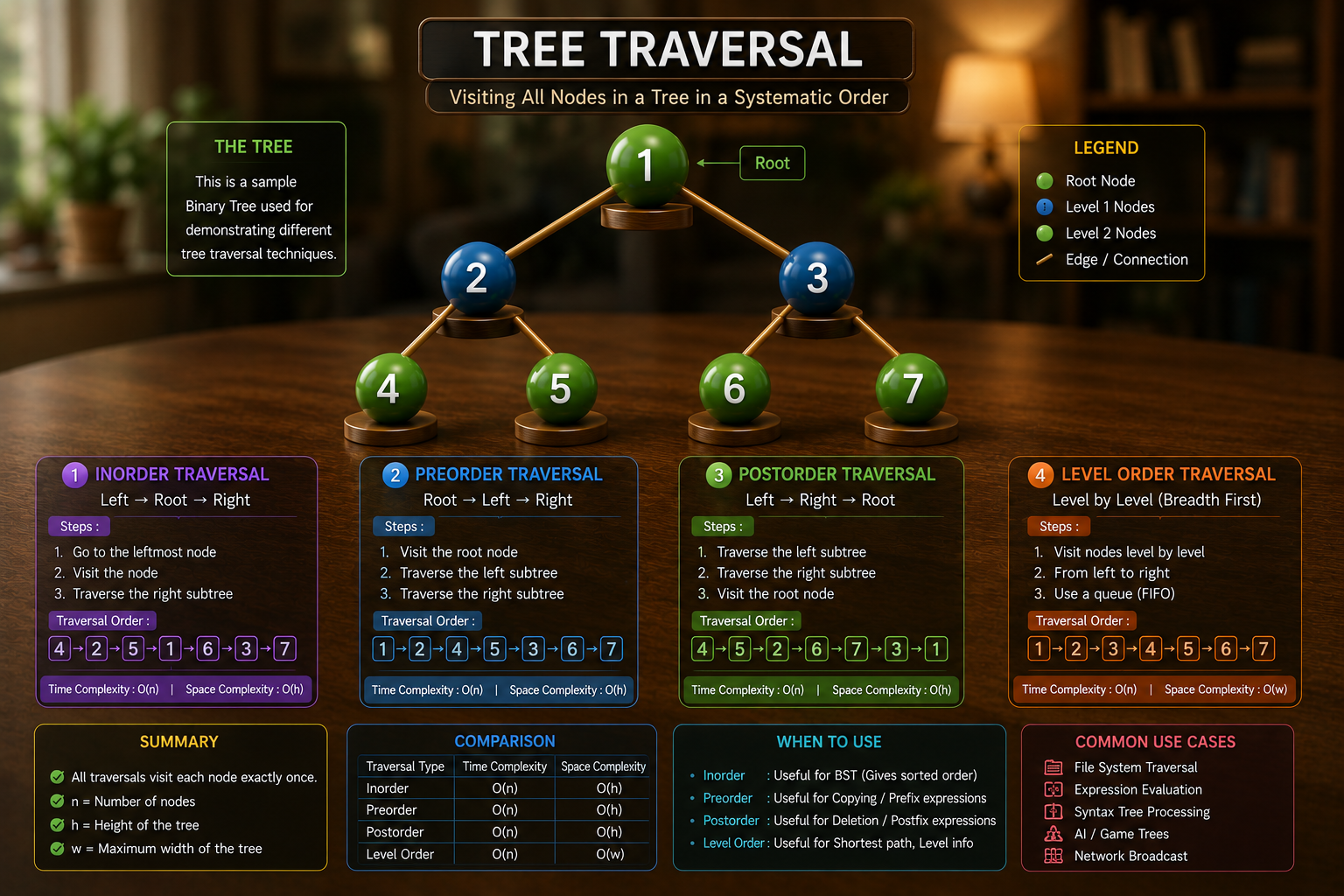
Tree Traverse
Tree traversal is the process of visiting every node in a tree exactly once in a specific order.
Tree traversals fall into two categories.
                  Tree Traversal
                       │
           ┌───────────┴───────────┐
           │                       │
          DFS                     BFS
           │                       │
   ┌───────┼────────┐              │
   │       │        │              │
  Preorder Inorder Postorder   Level Order
  (RLR)    (LRR)   (LRR*)      (Queue)
| Traversal | Time | Space | Common Use Cases |
|---|---|---|---|
| Preorder | Copying trees, serialization, prefix expressions | ||
| Inorder | Binary Search Trees, sorted output | ||
| Postorder | Deleting trees, postfix expressions, freeing memory | ||
| Level Order | Shortest path by levels, printing trees, BFS algorithms |
Where:
- n = number of nodes
- h = height of the tree
- w = maximum width of the tree
1. Depth-First Search (DFS) ↕️
Explore one branch completely before moving to another.
1.1 Preorder
Root → Left → Right
Traverse Root First then Left & right
50 → 30 → 20 → 40 → 35 → 45 → 70 → 60 → 80 → 90
flowchart LR
  N50(("50")) --> N30(("30"))
  N30 --> N20(("20"))
  N20 --> N40(("40"))
  N40 --> N35(("35"))
  N35 --> N45(("45"))
  N45 --> N70(("70"))
  N70 --> N60(("60"))
  N60 --> N80(("80"))
  N80 --> N90(("90"))

%% Root
  style N50 fill:#10B981,stroke:#047857,stroke-width:3px,color:#ffffff

%% Internal Nodes
  style N30 fill:#3B82F6,stroke:#1D4ED8,stroke-width:2px,color:#ffffff
  style N40 fill:#3B82F6,stroke:#1D4ED8,stroke-width:2px,color:#ffffff
  style N70 fill:#3B82F6,stroke:#1D4ED8,stroke-width:2px,color:#ffffff
  style N80 fill:#3B82F6,stroke:#1D4ED8,stroke-width:2px,color:#ffffff

%% Leaf Nodes
  style N20 fill:#F59E0B,stroke:#B45309,stroke-width:2px,color:#ffffff
  style N35 fill:#F59E0B,stroke:#B45309,stroke-width:2px,color:#ffffff
  style N45 fill:#F59E0B,stroke:#B45309,stroke-width:2px,color:#ffffff
  style N60 fill:#F59E0B,stroke:#B45309,stroke-width:2px,color:#ffffff
  style N90 fill:#F59E0B,stroke:#B45309,stroke-width:2px,color:#ffffff

%% Traversal path
  linkStyle default stroke:#EF4444,stroke-width:3px
1.2 Inorder
Left → Root → Right
💡Note: inorder traversal of a Binary Search Tree (BST) always visits the nodes in ascending sorted order.
20 → 30 → 35 → 40 → 45 → 50 → 60 → 70 → 80 → 90
flowchart LR
    N20(("20")) --> N30(("30"))
    N30 --> N35(("35"))
    N35 --> N40(("40"))
    N40 --> N45(("45"))
    N45 --> N50(("50"))
    N50 --> N60(("60"))
    N60 --> N70(("70"))
    N70 --> N80(("80"))
    N80 --> N90(("90"))

    %% Root
    style N50 fill:#10B981,stroke:#047857,stroke-width:3px,color:#ffffff

    %% Internal Nodes
    style N30 fill:#3B82F6,stroke:#1D4ED8,stroke-width:2px,color:#ffffff
    style N40 fill:#3B82F6,stroke:#1D4ED8,stroke-width:2px,color:#ffffff
    style N70 fill:#3B82F6,stroke:#1D4ED8,stroke-width:2px,color:#ffffff
    style N80 fill:#3B82F6,stroke:#1D4ED8,stroke-width:2px,color:#ffffff

    %% Leaf Nodes
    style N20 fill:#F59E0B,stroke:#B45309,stroke-width:2px,color:#ffffff
    style N35 fill:#F59E0B,stroke:#B45309,stroke-width:2px,color:#ffffff
    style N45 fill:#F59E0B,stroke:#B45309,stroke-width:2px,color:#ffffff
    style N60 fill:#F59E0B,stroke:#B45309,stroke-width:2px,color:#ffffff
    style N90 fill:#F59E0B,stroke:#B45309,stroke-width:2px,color:#ffffff

    %% Traversal path
    linkStyle default stroke:#10B981,stroke-width:3px
1.2 Postorder
Left → Right → Root
💡 Postorder is ideal when child nodes must be processed before their parent, such as deleting a tree, freeing memory, or evaluating expression trees from the bottom up.
20 → 35 → 45 → 40 → 30 → 60 → 90 → 80 → 70 → 50
flowchart LR
    N20(("20")) --> N35(("35"))
    N35 --> N45(("45"))
    N45 --> N40(("40"))
    N40 --> N30(("30"))
    N30 --> N60(("60"))
    N60 --> N90(("90"))
    N90 --> N80(("80"))
    N80 --> N70(("70"))
    N70 --> N50(("50"))

    %% Root
    style N50 fill:#10B981,stroke:#047857,stroke-width:3px,color:#ffffff

    %% Internal Nodes
    style N30 fill:#3B82F6,stroke:#1D4ED8,stroke-width:2px,color:#ffffff
    style N40 fill:#3B82F6,stroke:#1D4ED8,stroke-width:2px,color:#ffffff
    style N70 fill:#3B82F6,stroke:#1D4ED8,stroke-width:2px,color:#ffffff
    style N80 fill:#3B82F6,stroke:#1D4ED8,stroke-width:2px,color:#ffffff

    %% Leaf Nodes
    style N20 fill:#F59E0B,stroke:#B45309,stroke-width:2px,color:#ffffff
    style N35 fill:#F59E0B,stroke:#B45309,stroke-width:2px,color:#ffffff
    style N45 fill:#F59E0B,stroke:#B45309,stroke-width:2px,color:#ffffff
    style N60 fill:#F59E0B,stroke:#B45309,stroke-width:2px,color:#ffffff
    style N90 fill:#F59E0B,stroke:#B45309,stroke-width:2px,color:#ffffff

    %% Traversal path
    linkStyle default stroke:#F97316,stroke-width:3px
2. Breadth-First Search (BFS) ↔️
Visit nodes level by level using a queue
2.1 Level Order Traversal.
BFS is ideal for finding the shortest path in an unweighted tree or graph, pri
BFS (Level Order Traversal) uses a Queue (FIFO) to visit nodes level by level.
50 → 30 → 70 → 20 → 40 → 60 → 80 → 35 → 45 → 90
💡 It is commonly used for shortest-path problems in unweighted graphs, level-based processing, and tree serialization.
flowchart LR
    N50(("50")) --> N30(("30"))
    N30 --> N70(("70"))
    N70 --> N20(("20"))
    N20 --> N40(("40"))
    N40 --> N60(("60"))
    N60 --> N80(("80"))
    N80 --> N35(("35"))
    N35 --> N45(("45"))
    N45 --> N90(("90"))

    %% Root
    style N50 fill:#10B981,stroke:#047857,stroke-width:3px,color:#ffffff

    %% Internal Nodes
    style N30 fill:#3B82F6,stroke:#1D4ED8,stroke-width:2px,color:#ffffff
    style N40 fill:#3B82F6,stroke:#1D4ED8,stroke-width:2px,color:#ffffff
    style N70 fill:#3B82F6,stroke:#1D4ED8,stroke-width:2px,color:#ffffff
    style N80 fill:#3B82F6,stroke:#1D4ED8,stroke-width:2px,color:#ffffff

    %% Leaf Nodes
    style N20 fill:#F59E0B,stroke:#B45309,stroke-width:2px,color:#ffffff
    style N35 fill:#F59E0B,stroke:#B45309,stroke-width:2px,color:#ffffff
    style N45 fill:#F59E0B,stroke:#B45309,stroke-width:2px,color:#ffffff
    style N60 fill:#F59E0B,stroke:#B45309,stroke-width:2px,color:#ffffff
    style N90 fill:#F59E0B,stroke:#B45309,stroke-width:2px,color:#ffffff

    %% Traversal path
    linkStyle default stroke:#8B5CF6,stroke-width:3px
Skewed BST
Insert already-sorted data into a plain BST and every new node becomes the right child of the last one
- it degenerates into a linked list wearing a tree's name:
Now every operation is . This degeneration is the reason balanced trees exist.
This forms the basis of self-balancing trees such as AVL and Red-Black Trees
BALANCED BINARY SEARCH TREE (Balanced BST) ⚖️
A Balanced Binary Search Tree (Balanced BST) is a Binary Search Tree whose height remains approximately O(logn), ensuring efficient search, insertion, and deletion operations.
- Maintains BST ordering (Left < Root < Right)
- Height remains approximately
- Prevents degeneration into a linked list
- Guarantees efficient search, insertion, and deletion
Unlike a regular BST, a Balanced BST prevents the tree from becoming skewed.
The guarantee isn't free — every mutation may trigger rebalancing work — but it's still ,
and it's what backs ordered maps/sets in real libraries (std::map, Java TreeMap).
Reach for these whenever you need sorted iteration or range queries, which a hash table can't give you.
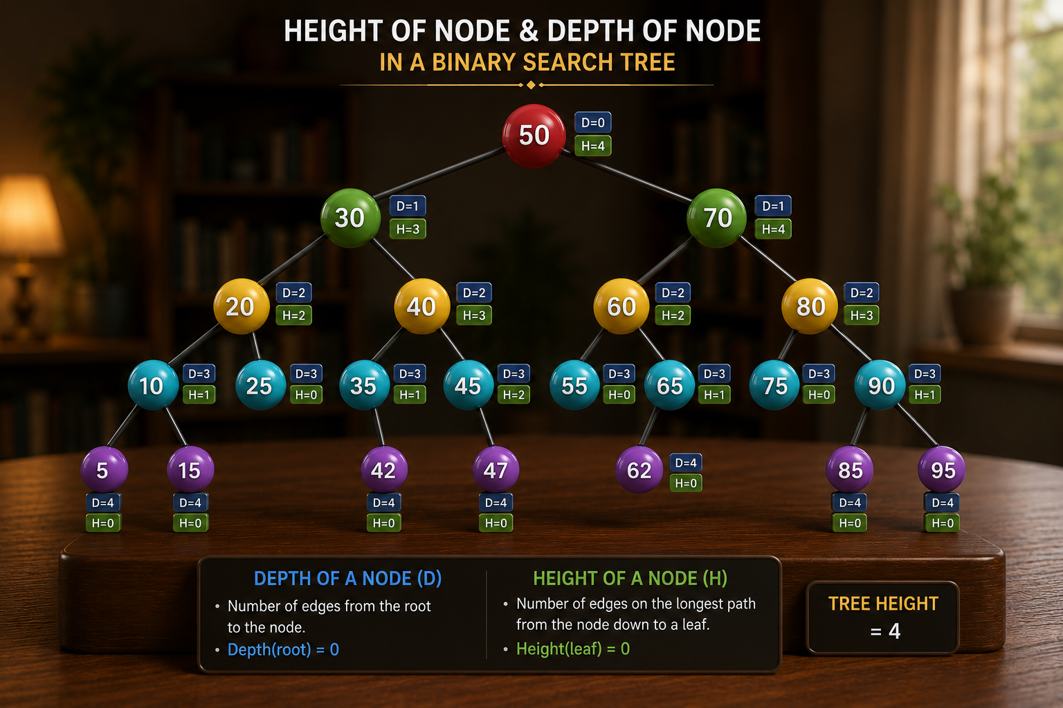
📐 height of a node
The height of a node is the number of edges on the longest path from that node to a leaf.
- Depth measures the distance from the root down to a node. (Top to Node)
- Height measures the distance from a node down to its deepest leaf. (Node to Bottom Leaf)
Formula
\text{Height(Node)} = 1 + \max(\text{Height(Left_tree)}, \text{Height(Right_tree)})
-
This way we can apply iteration
-
The height of a tree is the height of its root.
-
For a leaf node:
\text{Height_leaf} = 0
- A smaller height means fewer comparisons and faster operations.
Example Calculation
For node 40:
Height(35) = 0
Height(45) = 0

Height(40)
= 1 + max(0, 0)
= 1
For the root 50:
Height(30) = 2
Height(70) = 2

Height(50)
= 1 + max(2, 2)
= 3
Or calculate Maximize edges to farthest leaf
| Node | Height | comment |
|---|---|---|
| 35 | 0 | Leaf Node |
| 45 | 0 | Leaf Node |
| 75 | 0 | Leaf Node |
| 90 | 0 | Leaf Node |
| 20 | 0 | Leaf Node |
| 60 | 0 | Leaf Node |
| 40 | 1 | {40-35, 40-45} |
| 80 | 1 | {80-75, 80-90} |
| 30 | 2 | {30-20, 30-40-35, 30-40-45} |
| 70 | 2 | {70-60, 70-80-75, 70-80-90} |
| 50 | 3 | {50-30-20, 50-30-40-35, 50-30-40-45, 50-70-80-75} |
Balance Factor (BF) ⚖️
All node have a Balance Factor
BF = \text{Height(Left Subtree)} - \text{Height(Right Subtree)} }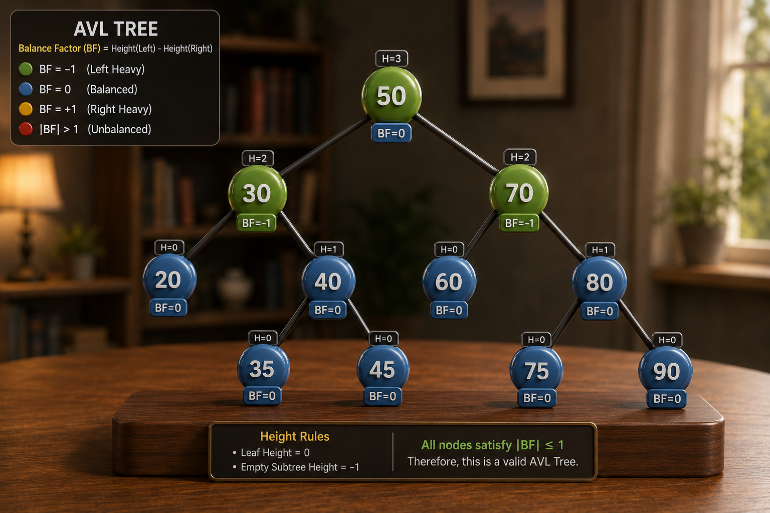
A node is considered balanced when:
or equivalently,
A node becomes unbalanced when:
Weight meaning
| Balance Factor | Status | Action |
|---|---|---|
| ✅ Balanced | None | |
| ✅ Balanced | None | |
| ✅ Balanced | None | |
| ❌ Right Heavy | RR or RL Rotation | |
| ❌ Left Heavy | LL or LR Rotation |
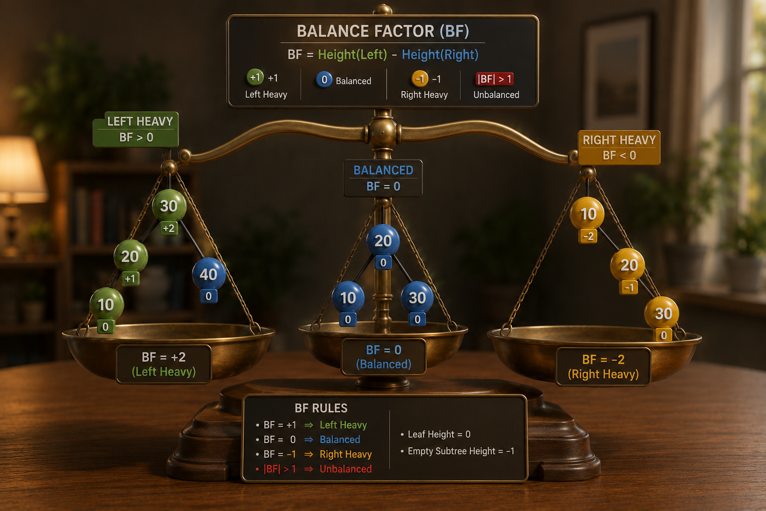
Left Heavy
A node is Left Heavy when its left subtree is taller than its right subtree.
the node is Left Heavy and requires either:
- LL Rotation
- LR Rotation
Right Heavy
A node is Right Heavy when its right subtree is taller than its left subtree.
the node is Right Heavy and requires either:
- RR Rotation
- RL Rotation
Examples of Balanced BSTs
- 🌿 AVL Tree
- 🔴⚫ Red-Black Tree
- 🌲 B-Tree
- 🌳 B+ Tree
- 🌐 Treap
- 🎲 Splay Tree (self-adjusting rather than strictly balanced)
AVL Tree
An AVL Tree is a self-balancing Binary Search Tree (BST) that automatically keeps its height balanced after every insertion and deletion.
It was invented by Georgy Adelson-Velsky and Evgenii Landis in 1962, making it the first self-balancing BST.
When Does a Rotation Occur? 🔄
A rotation is performed only after an insertion or deletion causes a node to become unbalanced.
The AVL tree follows these steps:
1. Insert/Delete Like a BST
Perform the normal Binary Search Tree (BST) insertion or deletion.
- Insert Smaller → Left Tree
- Insert Greater → Right Tree
No balancing is performed during the insertion itself.
2. Update Heights
Recalculate & update heights of each ancestor.
3. Calculate the Balance Factor (BF).
For every ancestor:
A node is balanced when
Otherwise,
and a rotation is required.
4. The rotation is performed at the first unbalanced ancestor.
After the appropriate rotation, the AVL tree regains its balanced height of approximately:
First Unbalanced Ancestor 🤸🏻♂️
The first ancestor whose balance factor becomes:
An AVL tree does not rebalance every node.
Instead, it starts at the modified node and moves upward toward the root, updating heights and checking the balance factor at each ancestor.
This is the only node that needs to be rotated after an insertion. Once it is rebalanced, the entire tree becomes balanced again.
Example Suppose we have this tree
flowchart TB
    N50(("50"))

    N50 --> N30(("30"))
    N50 --> N70(("70"))

    N30 --> N20(("20"))
    N30 --> N40(("40"))

    N70 --> N60(("60"))
    N70 --> N80(("80"))

    %% Extra nodes
    N40 --> N35(("35"))
    N40 --> N45(("45"))

    N80 --> N90(("90"))

    %% Root
    style N50 fill:#10B981,stroke:#047857,stroke-width:3px,color:#ffffff

    %% Internal Nodes
    style N30 fill:#3B82F6,stroke:#1D4ED8,stroke-width:2px,color:#ffffff
    style N70 fill:#3B82F6,stroke:#1D4ED8,stroke-width:2px,color:#ffffff
    style N40 fill:#3B82F6,stroke:#1D4ED8,stroke-width:2px,color:#ffffff
    style N80 fill:#3B82F6,stroke:#1D4ED8,stroke-width:2px,color:#ffffff

    %% Leaf Nodes
    style N20 fill:#F59E0B,stroke:#B45309,stroke-width:2px,color:#ffffff
    style N60 fill:#F59E0B,stroke:#B45309,stroke-width:2px,color:#ffffff
    style N35 fill:#F59E0B,stroke:#B45309,stroke-width:2px,color:#ffffff
    style N45 fill:#F59E0B,stroke:#B45309,stroke-width:2px,color:#ffffff
    style N90 fill:#F59E0B,stroke:#B45309,stroke-width:2px,color:#ffffff

    %% Edge styling
    linkStyle default stroke:#64748B,stroke-width:2px
Its a Balanced AVL tree
flowchart TB
    N50["<b>50</b><br/>H=3 | BF=0"]

    N50 --> N30["30<br/>H=2 | BF=-1"]
    N50 --> N70["70<br/>H=2 | BF=-1"]

    N30 --> N20["20<br/>H=0 | BF=0"]
    N30 --> N40["40<br/>H=1 | BF=0"]

    N70 --> N60["60<br/>H=0 | BF=0"]
    N70 --> N80["80<br/>H=1 | BF=-1"]

    N40 --> N35["35<br/>H=0 | BF=0"]
    N40 --> N45["45<br/>H=0 | BF=0"]

    N80 --> N90["90<br/>H=0 | BF=0"]

    %% Root
    style N50 fill:#10B981,stroke:#047857,stroke-width:3px,color:#ffffff

    %% Internal Nodes
    style N30 fill:#3B82F6,stroke:#1D4ED8,stroke-width:2px,color:#ffffff
    style N70 fill:#3B82F6,stroke:#1D4ED8,stroke-width:2px,color:#ffffff
    style N40 fill:#3B82F6,stroke:#1D4ED8,stroke-width:2px,color:#ffffff
    style N80 fill:#3B82F6,stroke:#1D4ED8,stroke-width:2px,color:#ffffff

    %% Leaf Nodes
    style N20 fill:#F59E0B,stroke:#B45309,stroke-width:2px,color:#ffffff
    style N60 fill:#F59E0B,stroke:#B45309,stroke-width:2px,color:#ffffff
    style N35 fill:#F59E0B,stroke:#B45309,stroke-width:2px,color:#ffffff
    style N45 fill:#F59E0B,stroke:#B45309,stroke-width:2px,color:#ffffff
    style N90 fill:#F59E0B,stroke:#B45309,stroke-width:2px,color:#ffffff

    %% Edge styling
    linkStyle default stroke:#64748B,stroke-width:2px
This can be visualized as:
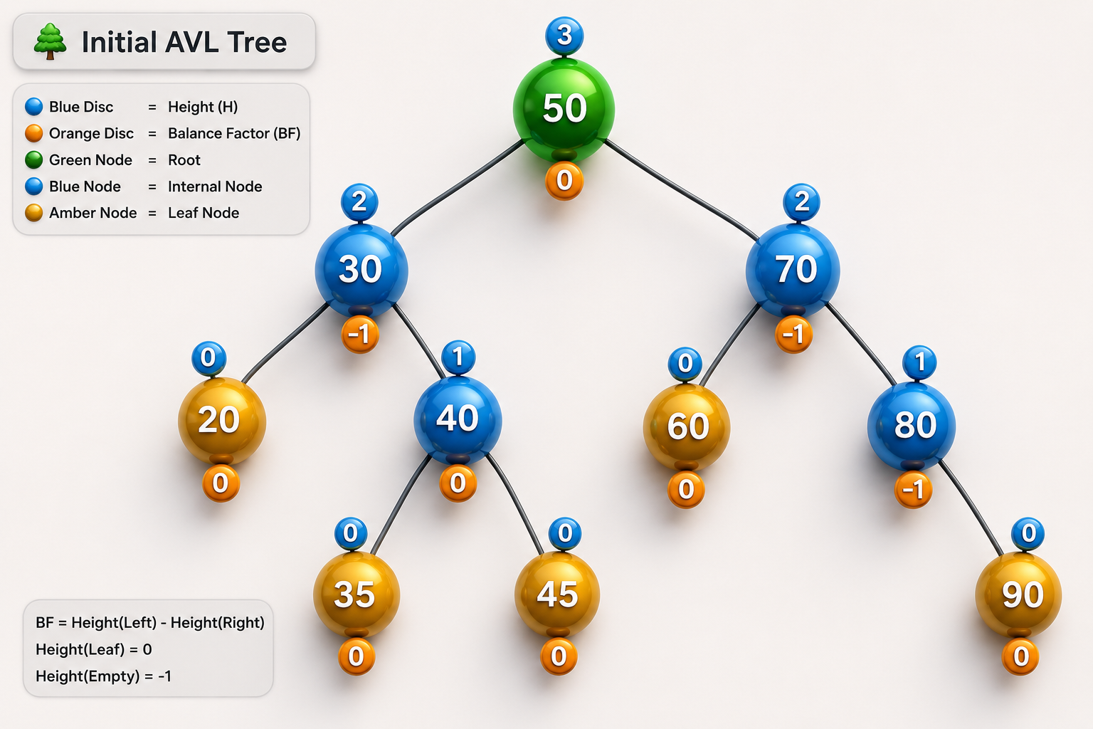
AVL rotation cases
Think of the two letters as directions you follow from the first unbalanced ancestor to reach the newly inserted node:
First Letter → Which side of the first unbalanced node is taller.
- L = Left subtree (BF > 1)
- R = Right subtree (BF < -1)
Second Letter → Which side of that child contains the inserted node (or taller subtree).
- L = Left subtree
- R = Right subtree
The Four AVL Cases
| Case | Insertion Path | Rotation |
|---|---|---|
| LL | Left → Left | Right Rotation ⤵️ |
| RR | Right → Right | Left Rotation |
| LR | Left → Right | Left Rotation → Right Rotation |
| RL | Right → Left | Right Rotation → Left Rotation |
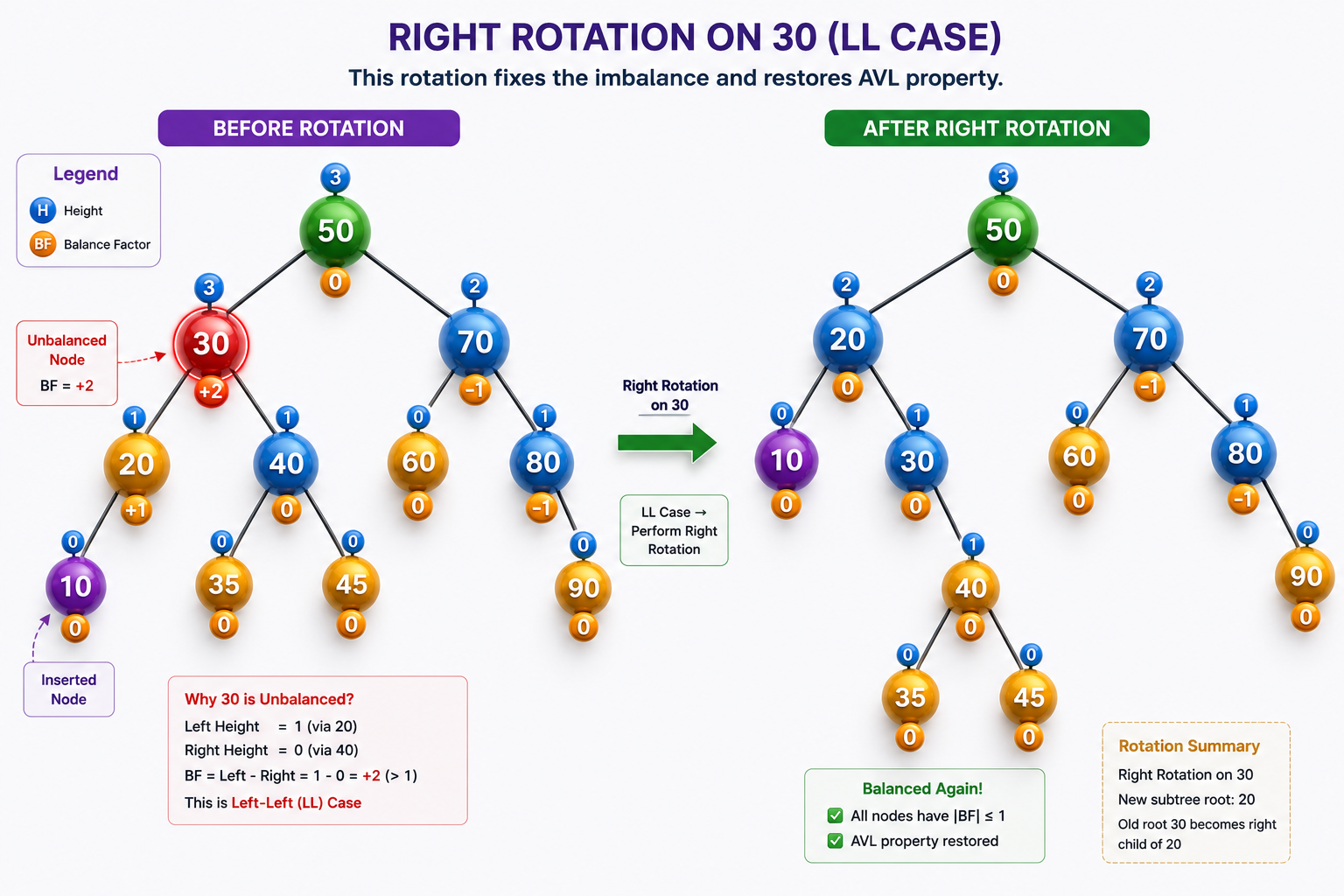
1. LL Rotation on Insertion
Condition
- Node is Left Heavy
- New node inserted into the left subtree of the left child
Example:
Lets insert 10 on Left subtree
It will make left subtree heavier & imbalanced at ancestor 30
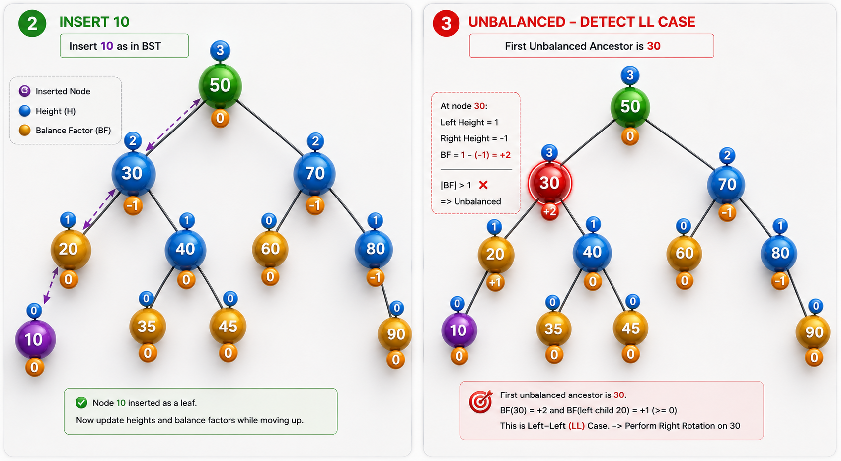
To balance the tree we need to perform right rotation ⤵️
flowchart LR

subgraph Before["Before Right Rotation"]
direction TB

Y(("y"))
X(("x"))
T3(("T3"))
T1(("T1"))
T2(("T2"))

Y --> X
Y --> T3

X --> T1
X --> T2
end

R["⤵️ Right Rotation"]

subgraph After["After Right Rotation"]
direction TB

X2(("x"))
T12(("T1"))
Y2(("y"))
T22(("T2"))
T32(("T3"))

X2 --> T12
X2 --> Y2

Y2 --> T22
Y2 --> T32
end

Before --> R --> After

%% Before colors
style Y fill:#EF4444,stroke:#B91C1C,stroke-width:3px,color:#fff
style X fill:#3B82F6,stroke:#1D4ED8,stroke-width:2px,color:#fff
style T1 fill:#F59E0B,stroke:#B45309,color:#fff
style T2 fill:#F59E0B,stroke:#B45309,color:#fff
style T3 fill:#F59E0B,stroke:#B45309,color:#fff

%% After colors
style X2 fill:#10B981,stroke:#047857,stroke-width:3px,color:#fff
style Y2 fill:#3B82F6,stroke:#1D4ED8,stroke-width:2px,color:#fff
style T12 fill:#F59E0B,stroke:#B45309,color:#fff
style T22 fill:#F59E0B,stroke:#B45309,color:#fff
style T32 fill:#F59E0B,stroke:#B45309,color:#fff

linkStyle default stroke:#64748B,stroke-width:2px
Where:
- x = left child (pivot)
- y = unbalanced node
- T1, T2, T3 = subtrees that remain in BST order
This is why rotations are O(1): regardless of the tree size, they only update a constant number of parent and child references while preserving the BST property.
Now we need to perform right rotation at 20 to move heavier node on right.
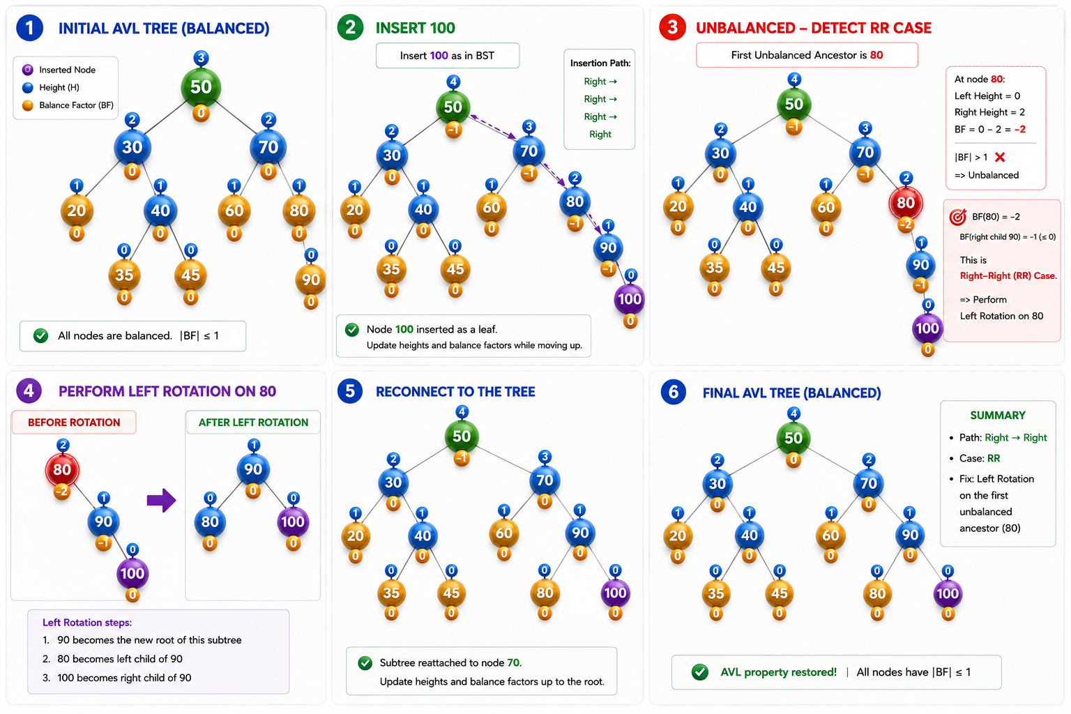
2. RR Rotation on Insertion ↪️
Condition
- Node is Right Heavy
- New node inserted into the right subtree of the right child
Example: Lets insert 100 on right subtree
It will make right subtree heavier & imbalanced at ancestor 80
To balance the tree we need to perform left rotation ↪️
flowchart LR

subgraph Before["Before Left Rotation"]
direction TB

X(("x"))
T1(("T1"))
Y(("y"))
T2(("T2"))
T3(("T3"))

X --> T1
X --> Y

Y --> T2
Y --> T3
end

R["⤴️ Left Rotation"]

subgraph After["After Left Rotation"]
direction TB

Y2(("y"))
X2(("x"))
T32(("T3"))
T12(("T1"))
T22(("T2"))

Y2 --> X2
Y2 --> T32

X2 --> T12
X2 --> T22
end

Before --> R --> After

%% Before colors
style X fill:#EF4444,stroke:#B91C1C,stroke-width:3px,color:#fff
style Y fill:#3B82F6,stroke:#1D4ED8,stroke-width:2px,color:#fff
style T1 fill:#F59E0B,stroke:#B45309,color:#fff
style T2 fill:#F59E0B,stroke:#B45309,color:#fff
style T3 fill:#F59E0B,stroke:#B45309,color:#fff

%% After colors
style Y2 fill:#10B981,stroke:#047857,stroke-width:3px,color:#fff
style X2 fill:#3B82F6,stroke:#1D4ED8,stroke-width:2px,color:#fff
style T12 fill:#F59E0B,stroke:#B45309,color:#fff
style T22 fill:#F59E0B,stroke:#B45309,color:#fff
style T32 fill:#F59E0B,stroke:#B45309,color:#fff

linkStyle default stroke:#64748B,stroke-width:2px
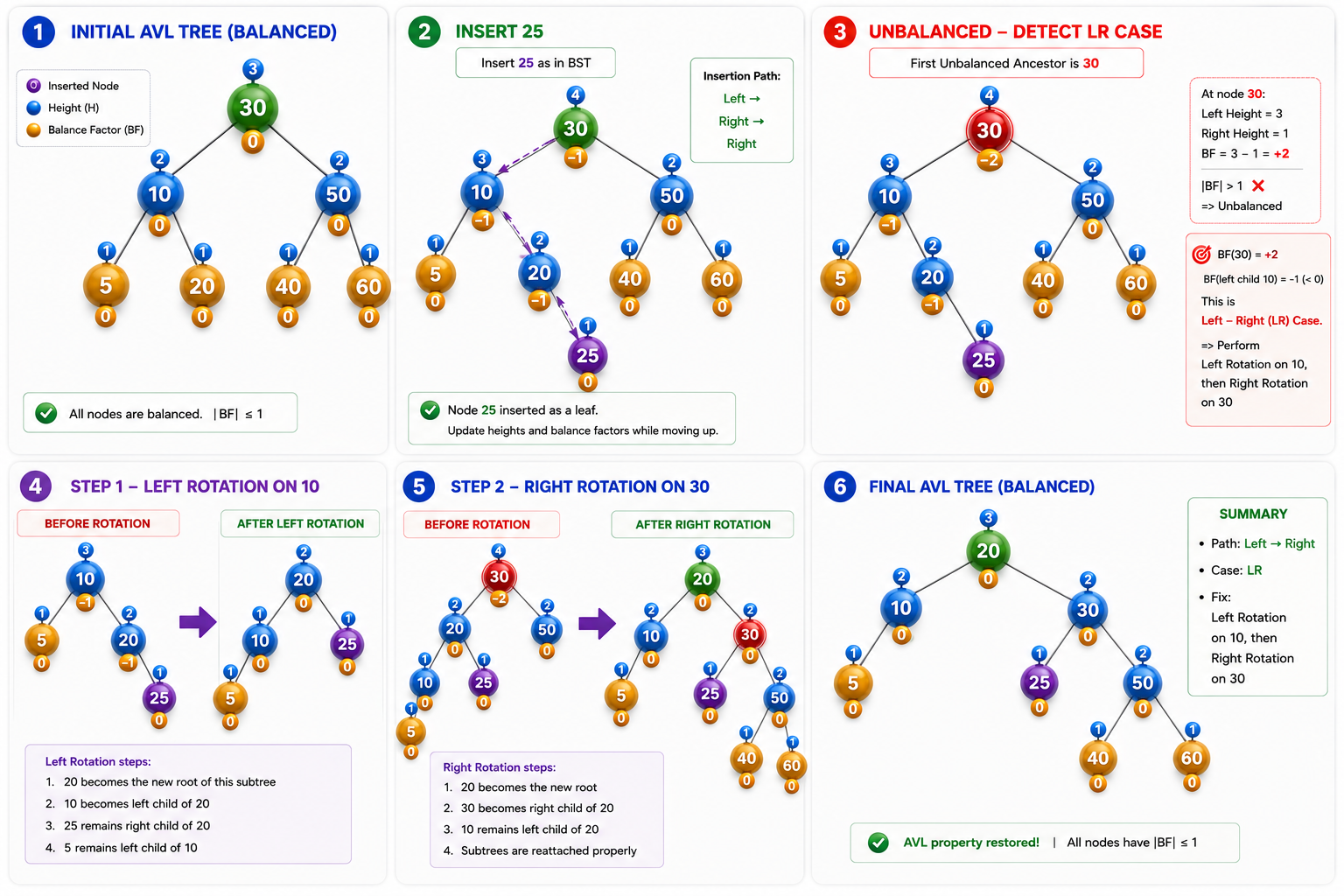
3. LR Rotation on Insertion ↪️
Condition
- Node is Left Heavy
- New node inserted into the right subtree of the left child
Example:
Lets insert 100 on right subtree
flowchart LR

subgraph Before["Before LR Rotation"]
direction TB

Z(("z"))
X(("x"))
T4(("T4"))
T1(("T1"))
Y(("y"))
T2(("T2"))
T3(("T3"))

Z --> X
Z --> T4

X --> T1
X --> Y

Y --> T2
Y --> T3
end

R1["⤴️ Left Rotation<br/>on x"]

subgraph Middle["Intermediate"]
direction TB

Z2(("z"))
Y2(("y"))
T42(("T4"))
X2(("x"))
T22(("T2"))
T12(("T1"))
T32(("T3"))

Z2 --> Y2
Z2 --> T42

Y2 --> X2
Y2 --> T32

X2 --> T12
X2 --> T22
end

R2["⤵️ Right Rotation<br/>on z"]

subgraph After["After LR Rotation"]
direction TB

Y3(("y"))
X3(("x"))
Z3(("z"))
T13(("T1"))
T23(("T2"))
T33(("T3"))
T43(("T4"))

Y3 --> X3
Y3 --> Z3

X3 --> T13
X3 --> T23

Z3 --> T33
Z3 --> T43
end

Before --> R1 --> Middle --> R2 --> After

%% Before
style Z fill:#EF4444,stroke:#B91C1C,stroke-width:3px,color:#fff
style X fill:#3B82F6,stroke:#1D4ED8,color:#fff
style Y fill:#8B5CF6,stroke:#6D28D9,color:#fff

%% Middle
style Z2 fill:#EF4444,stroke:#B91C1C,stroke-width:3px,color:#fff
style X2 fill:#3B82F6,stroke:#1D4ED8,color:#fff
style Y2 fill:#8B5CF6,stroke:#6D28D9,color:#fff

%% After
style Y3 fill:#10B981,stroke:#047857,stroke-width:3px,color:#fff
style X3 fill:#3B82F6,stroke:#1D4ED8,color:#fff
style Z3 fill:#3B82F6,stroke:#1D4ED8,color:#fff

%% Subtrees
style T1 fill:#F59E0B,stroke:#B45309,color:#fff
style T2 fill:#F59E0B,stroke:#B45309,color:#fff
style T3 fill:#F59E0B,stroke:#B45309,color:#fff
style T4 fill:#F59E0B,stroke:#B45309,color:#fff

style T12 fill:#F59E0B,stroke:#B45309,color:#fff
style T22 fill:#F59E0B,stroke:#B45309,color:#fff
style T32 fill:#F59E0B,stroke:#B45309,color:#fff
style T42 fill:#F59E0B,stroke:#B45309,color:#fff

style T13 fill:#F59E0B,stroke:#B45309,color:#fff
style T23 fill:#F59E0B,stroke:#B45309,color:#fff
style T33 fill:#F59E0B,stroke:#B45309,color:#fff
style T43 fill:#F59E0B,stroke:#B45309,color:#fff

linkStyle default stroke:#64748B,stroke-width:2px
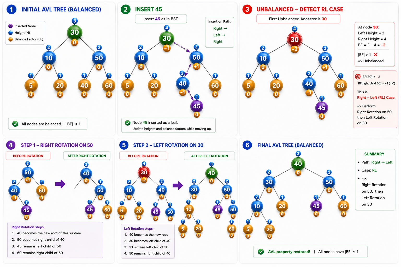
4. RL Rotation on Insertion ↪️
Condition
- Node is Right Heavy
- New node inserted into the left subtree of the right child
Example: Lets insert 100 on right subtree
flowchart LR

subgraph Before["Before RL Rotation"]
direction TB

Z(("z"))
T1(("T1"))
X(("x"))
Y(("y"))
T4(("T4"))
T2(("T2"))
T3(("T3"))

Z --> T1
Z --> X

X --> Y
X --> T4

Y --> T2
Y --> T3
end

R1["⤵️ Right Rotation<br/>on x"]

subgraph Middle["Intermediate"]
direction TB

Z2(("z"))
T12(("T1"))
Y2(("y"))
T22(("T2"))
X2(("x"))
T32(("T3"))
T42(("T4"))

Z2 --> T12
Z2 --> Y2

Y2 --> T22
Y2 --> X2

X2 --> T32
X2 --> T42
end

R2["⤴️ Left Rotation<br/>on z"]

subgraph After["After RL Rotation"]
direction TB

Y3(("y"))
Z3(("z"))
X3(("x"))
T13(("T1"))
T23(("T2"))
T33(("T3"))
T43(("T4"))

Y3 --> Z3
Y3 --> X3

Z3 --> T13
Z3 --> T23

X3 --> T33
X3 --> T43
end

Before --> R1 --> Middle --> R2 --> After

%% Before
style Z fill:#EF4444,stroke:#B91C1C,stroke-width:3px,color:#fff
style X fill:#3B82F6,stroke:#1D4ED8,color:#fff
style Y fill:#8B5CF6,stroke:#6D28D9,color:#fff

%% Middle
style Z2 fill:#EF4444,stroke:#B91C1C,stroke-width:3px,color:#fff
style X2 fill:#3B82F6,stroke:#1D4ED8,color:#fff
style Y2 fill:#8B5CF6,stroke:#6D28D9,color:#fff

%% After
style Y3 fill:#10B981,stroke:#047857,stroke-width:3px,color:#fff
style Z3 fill:#3B82F6,stroke:#1D4ED8,color:#fff
style X3 fill:#3B82F6,stroke:#1D4ED8,color:#fff

%% Subtrees
style T1 fill:#F59E0B,stroke:#B45309,color:#fff
style T2 fill:#F59E0B,stroke:#B45309,color:#fff
style T3 fill:#F59E0B,stroke:#B45309,color:#fff
style T4 fill:#F59E0B,stroke:#B45309,color:#fff

style T12 fill:#F59E0B,stroke:#B45309,color:#fff
style T22 fill:#F59E0B,stroke:#B45309,color:#fff
style T32 fill:#F59E0B,stroke:#B45309,color:#fff
style T42 fill:#F59E0B,stroke:#B45309,color:#fff

style T13 fill:#F59E0B,stroke:#B45309,color:#fff
style T23 fill:#F59E0B,stroke:#B45309,color:#fff
style T33 fill:#F59E0B,stroke:#B45309,color:#fff
style T43 fill:#F59E0B,stroke:#B45309,color:#fff

linkStyle default stroke:#64748B,stroke-width:2px
AVL Tree Properties
AVL Trees provide the fastest search performance among common self-balancing binary search trees by maintaining a very strict balance.
| Operation | Time Complexity |
|---|---|
| 🔍 Search | |
| ➕ Insert | |
| 🗑️ Delete | |
| 🌳 Traversal (Inorder, Preorder, Postorder, BFS) |
Overhead
The trade-off is more rotations, additional metadata, and greater implementation complexity, making them less suitable for update-heavy workloads.
| Operation | Time Complexity |
|---|---|
| 🔄 Single Rotation (LL, RR) | |
| 🔁 Double Rotation (LR, RL) | |
| 📏 Height Calculation | (stored in each node) |
| ⚖️ Balance Factor Update |
Comparison with BST
| Operation | Binary Search Tree | AVL Tree |
|---|---|---|
| Search | Worst: | |
| Insert | Worst: | |
| Delete | Worst: | |
| Height | Worst: | |
| Rotation | ❌ |
where
- h: is height of tree
- n: number of nodes
✅ AVL Tree Advantages
- Guaranteed height of
- Fast searching
- Predictable performance
- Ideal for read-heavy workloads
❌ AVL Tree Limitations
- More rotations than Red-Black Trees
- Extra memory for height or balance factor
- More complex implementation
Problems with AVL Trees
- Frequent Rotations Overhead
AVL Trees rebalance after every insertion and deletion.
-
Deletion can even trigger multiple rotations while moving toward the root.
-
Not Ideal for Write-Heavy Workloads
- Complexity
AVL Trees require maintaining:
Every insertion and deletion updates metadata.
- Height
- Balance Factor
- Four rotation cases
- Height updates after every modification
This makes AVL Trees significantly more complex than a standard BST.
🔴 Red-Black Tree
Red-Black Trees were designed to overcome the high maintenance cost of AVL Trees.
Because Red-Black Trees provide an excellent balance between search speed and update performance, they are widely used in production systems.
Examples:
- Linux Kernel (
rbtree) - Process schedulers
- Timer management
- Virtual memory management
AVL Tree vs RedBlack Tree
Although both have the same asymptotic complexity, their practical performance differs.
| Operation | AVL Tree | Red-Black Tree |
|---|---|---|
| 🔍 Search | ||
| ➕ Insert | ||
| ❌ Delete | ||
| 🌳 Traversal | ||
| 🔄 Rotation |
Rotations Comparison
AVL Trees spend more time rebalancing after updates.
| Operation | AVL Tree | Red-Black Tree |
|---|---|---|
| Insert | More Rotations | Fewer Rotations |
| Delete | May require Multiple Rotations | Usually Fewer Rotations |
Height Comparison
| Property | AVL Tree | Red-Black Tree |
|---|---|---|
| Balance | Strict | Relaxed |
| Maximum Height | Smaller | Slightly Taller |
| Search Path | Shorter | Slightly Longer |
AVL Trees maintain a lower height, so searches generally visit fewer nodes.
Instead of enforcing strict balance, it guarantees that no path is more than twice as long as any other.
- Maintains balance using five coloring rules.
Five Properties of a Red-Black Tree
A valid Red-Black Tree must satisfy the following five properties.
1. Every node is either RED 🔴 or BLACK ⚫
Each node has exactly one color 🔴 / ⚫
flowchart TB
    A(("20"))
    B(("10"))
    C(("30"))

    A --> B
    A --> C

    style A fill:#222,stroke:#000,stroke-width:2px,color:#fff
    style B fill:#E53935,stroke:#B71C1C,stroke-width:2px,color:#fff
    style C fill:#E53935,stroke:#B71C1C,stroke-width:2px,color:#fff
Why Colors?
The color determines whether rotations are needed.
🔴 Red
Red nodes are considered "flexible" nodes that don't contribute to the tree's black height.
- If consecutive red nodes were allowed, you could build a long chain like:
⚫ Black
Black nodes are considered "stable" nodes that contribute to the tree's black height.
- Having consecutive black nodes does not violate any property, as long as every root-to-leaf path contains the same number of black nodes.
No other colors are allowed.
2. The root is always Black.
The root node must always be Black.
- If an insertion creates a red root, it is simply recolored to black.
flowchart TD

subgraph VALID["✅ Valid"]
direction TB

A1(("20"))
B1(("10"))
C1(("30"))

A1 --> B1
A1 --> C1

style A1 fill:#222,stroke:#000,stroke-width:2px,color:#fff
style B1 fill:#E53935,stroke:#B71C1C,stroke-width:2px,color:#fff
style C1 fill:#E53935,stroke:#B71C1C,stroke-width:2px,color:#fff

end

subgraph INVALID["❌ Invalid"]
direction TB

A2(("20"))
B2(("10"))
C2(("30"))

A2 --> B2
A2 --> C2

style A2 fill:#E53935,stroke:#B71C1C,stroke-width:3px,color:#fff
style B2 fill:#222,stroke:#000,stroke-width:2px,color:#fff
style C2 fill:#222,stroke:#000,stroke-width:2px,color:#fff

end

linkStyle default stroke:#64748B,stroke-width:2px
3. Every leaf is Black.
Every missing child is represented by a special NIL node
Every NIL node is considered Black.
flowchart TB
    A(("20"))
    B(("10"))
    C(("30"))

    NIL1["NIL"]
    NIL2["NIL"]
    NIL3["NIL"]
    NIL4["NIL"]

    A --> B
    A --> C

    B --> NIL1
    B --> NIL2

    C --> NIL3
    C --> NIL4

    style A fill:#222,stroke:#000,color:#fff
    style B fill:#E53935,stroke:#B71C1C,color:#fff
    style C fill:#E53935,stroke:#B71C1C,color:#fff

    style NIL1 fill:#222,stroke:#000,color:#fff
    style NIL2 fill:#222,stroke:#000,color:#fff
    style NIL3 fill:#222,stroke:#000,color:#fff
    style NIL4 fill:#222,stroke:#000,color:#fff
Although these NIL nodes are usually not drawn, they are conceptually part of the tree and play a key role in maintaining the balancing properties.
4. Red Rule: A Red node cannot have a Red child.
Black nodes can have children of either color, but red nodes can only have black children.
It prevents long chains of red nodes that would make the tree unbalanced.
| Parent | Child | Allowed? |
|---|---|---|
| ⚫ Black | ⚫ Black | ✅ Yes |
| ⚫ Black | 🔴 Red | ✅ Yes |
| 🔴 Red | ⚫ Black | ✅ Yes |
| 🔴 Red | 🔴 Red | ❌ No |
flowchart TD


subgraph VALID["✅ Valid"]
direction TB

A1(("20"))
B1(("10"))
C1(("5"))

A1 --> B1
B1 --> C1

style A1 fill:#222,stroke:#000,color:#fff
style B1 fill:#E53935,stroke:#B71C1C,color:#fff
style C1 fill:#222,stroke:#000,color:#fff

end

subgraph INVALID["❌ Invalid"]
direction TB

A2(("20"))
B2(("10"))
C2(("5"))

A2 --> B2
B2 --> C2

style A2 fill:#222,stroke:#000,color:#fff
style B2 fill:#E53935,stroke:#B71C1C,color:#fff
style C2 fill:#E53935,stroke:#B71C1C,stroke-width:3px,color:#fff

end


subgraph VALID["✅ Valid"]
    direction TB

    A3(("20"))
    B3(("10"))
    C3(("5"))

    A3 --> B3
    B3 --> C3

    style A3 fill:#222,stroke:#000,color:#fff
    style B3 fill:#222,stroke:#000,color:#fff
    style C3 fill:#222,stroke:#000,color:#fff

end


subgraph VALID["✅ Valid"]
    direction TB

    A4(("20"))
    B4(("10"))
    C4(("5"))

    A4 --> B4
    B4 --> C4

    style A4 fill:#E53935,stroke:#000,color:#fff
    style B4 fill:#222,stroke:#000,color:#fff
    style C4 fill:#222,stroke:#000,color:#fff

end
5. Every Path Has the Same Number of Black Nodes ⚫
Every path from a node to any NIL leaf must contain the same number of Black nodes.
flowchart TB

    N50(("50"))

    N50 --> N30(("30"))
    N50 --> N70(("70"))

    N30 --> N20(("20"))
    N30 --> N40(("40"))

    N70 --> N60(("60"))
    N70 --> N90(("90"))

    N40 --> N35(("35"))
    N40 --> N45(("45"))

    N90 --> N80(("80"))

%% NIL Leaves
    N20 --> NIL1(("NIL"))
    N20 --> NIL2(("NIL"))

    N35 --> NIL3(("NIL"))
    N35 --> NIL4(("NIL"))

    N45 --> NIL5(("NIL"))
    N45 --> NIL6(("NIL"))

    N60 --> NIL7(("NIL"))
    N60 --> NIL8(("NIL"))

    N80 --> NIL9(("NIL"))
    N80 --> NIL10(("NIL"))

    N90 --> NIL11(("NIL"))

%% Black Nodes
    style N50 fill:#222222,stroke:#000000,stroke-width:3px,color:#ffffff
    style N20 fill:#222222,stroke:#000000,stroke-width:3px,color:#ffffff
    style N40 fill:#222222,stroke:#000000,stroke-width:3px,color:#ffffff
    style N60 fill:#222222,stroke:#000000,stroke-width:3px,color:#ffffff
    style N90 fill:#222222,stroke:#000000,stroke-width:3px,color:#ffffff

%% Red Nodes
    style N30 fill:#E53935,stroke:#B71C1C,stroke-width:3px,color:#ffffff
    style N70 fill:#E53935,stroke:#B71C1C,stroke-width:3px,color:#ffffff
    style N35 fill:#E53935,stroke:#B71C1C,stroke-width:3px,color:#ffffff
    style N45 fill:#E53935,stroke:#B71C1C,stroke-width:3px,color:#ffffff
    style N80 fill:#E53935,stroke:#B71C1C,stroke-width:3px,color:#ffffff

%% NIL Nodes
    style NIL1 fill:#222222,stroke:#000000,color:#ffffff
    style NIL2 fill:#222222,stroke:#000000,color:#ffffff
    style NIL3 fill:#222222,stroke:#000000,color:#ffffff
    style NIL4 fill:#222222,stroke:#000000,color:#ffffff
    style NIL5 fill:#222222,stroke:#000000,color:#ffffff
    style NIL6 fill:#222222,stroke:#000000,color:#ffffff
    style NIL7 fill:#222222,stroke:#000000,color:#ffffff
    style NIL8 fill:#222222,stroke:#000000,color:#ffffff
    style NIL9 fill:#222222,stroke:#000000,color:#ffffff
    style NIL10 fill:#222222,stroke:#000000,color:#ffffff
    style NIL11 fill:#222222,stroke:#000000,color:#ffffff

    linkStyle default stroke:#64748B,stroke-width:2px
Black Height
Black Height (BH) of a node is the number of black nodes on any path from (but not including) that node to a descendant NIL leaf, including the NIL leaf.
Include the NIL leaf
If node is RED: If node is BLACK:
flowchart TB

    N50["50<br/>BH = 2"]

    N50 --> N30["30<br/>BH = 1"]
    N50 --> N70["70<br/>BH = 1"]

    N30 --> N20["20<br/>BH = 1"]
    N30 --> N40["40<br/>BH = 1"]

    N70 --> N60["60<br/>BH = 1"]
    N70 --> N90["90<br/>BH = 1"]

    N40 --> N35["35<br/>BH = 0"]
    N40 --> N45["45<br/>BH = 0"]

    N90 --> N80["80<br/>BH = 0"]

%% NIL Leaves
    N20 --> NIL1["NIL<br/>BH = 0"]
    N20 --> NIL2["NIL<br/>BH = 0"]

    N35 --> NIL3["NIL<br/>BH = 0"]
    N35 --> NIL4["NIL<br/>BH = 0"]

    N45 --> NIL5["NIL<br/>BH = 0"]
    N45 --> NIL6["NIL<br/>BH = 0"]

    N60 --> NIL7["NIL<br/>BH = 0"]
    N60 --> NIL8["NIL<br/>BH = 0"]

    N80 --> NIL9["NIL<br/>BH = 0"]
    N80 --> NIL10["NIL<br/>BH = 0"]

    N90 --> NIL11["NIL<br/>BH = 0"]

%% Black Nodes
    style N50 fill:#222222,stroke:#000000,stroke-width:3px,color:#ffffff
    style N20 fill:#222222,stroke:#000000,stroke-width:3px,color:#ffffff
    style N40 fill:#222222,stroke:#000000,stroke-width:3px,color:#ffffff
    style N60 fill:#222222,stroke:#000000,stroke-width:3px,color:#ffffff
    style N90 fill:#222222,stroke:#000000,stroke-width:3px,color:#ffffff

%% Red Nodes
    style N30 fill:#E53935,stroke:#B71C1C,stroke-width:3px,color:#ffffff
    style N70 fill:#E53935,stroke:#B71C1C,stroke-width:3px,color:#ffffff
    style N35 fill:#E53935,stroke:#B71C1C,stroke-width:3px,color:#ffffff
    style N45 fill:#E53935,stroke:#B71C1C,stroke-width:3px,color:#ffffff
    style N80 fill:#E53935,stroke:#B71C1C,stroke-width:3px,color:#ffffff

%% NIL Nodes
    style NIL1 fill:#222222,stroke:#000000,color:#ffffff
    style NIL2 fill:#222222,stroke:#000000,color:#ffffff
    style NIL3 fill:#222222,stroke:#000000,color:#ffffff
    style NIL4 fill:#222222,stroke:#000000,color:#ffffff
    style NIL5 fill:#222222,stroke:#000000,color:#ffffff
    style NIL6 fill:#222222,stroke:#000000,color:#ffffff
    style NIL7 fill:#222222,stroke:#000000,color:#ffffff
    style NIL8 fill:#222222,stroke:#000000,color:#ffffff
    style NIL9 fill:#222222,stroke:#000000,color:#ffffff
    style NIL10 fill:#222222,stroke:#000000,color:#ffffff
    style NIL11 fill:#222222,stroke:#000000,color:#ffffff

    linkStyle default stroke:#64748B,stroke-width:2px
Both paths have the same Black Height.
This satisfies Property 5.
The longest root-to-leaf path can be at most twice the length of the shortest path.
Why Black Height Matters
Property 5 guarantees that every path from a node to its descendant NIL leaves contains the same number of black nodes.
Property 4 guarantees that two red nodes can never appear consecutively.
Therefore, between any two black nodes there can be at most one red node.
The longest possible path alternates
⚫ -- 🔴 -- ⚫ -- 🔴 -- ⚫
This means
The longest root-to-leaf path can be at most twice the length of the shortest path.
Suppose
- Height =
- Black Height =
Since red nodes cannot be adjacent,
the maximum possible height occurs when every black node has a red child.
Therefore
Searching In RedBlack Tree
Searching in a Red-Black Tree is identical to searching in a Binary Search Tree (BST).
The node colors are ignored during the search.
Only the BST ordering property is used.
Starting from the root:
- Compare the target value with the current node.
- If equal, return the node.
- If smaller, move to the left child.
- If larger, move to the right child.
- Repeat until the value is found or a NIL node is reached.
Pseudocode:
Node* search(Node* root, int key)
{
    while (root != nullptr)
    {
        if (key == root->value)
            return root;

        if (key < root->value)
            root = root->left;
        else
            root = root->right;
    }

    return nullptr;
}
Search Complexity of Red-Black Tree
| Operation | Complexity |
|---|---|
| Best Case | |
| Average Case | |
| Worst Case |
Inserting In Red Black Tree
- Insert the new node exactly like a BST.
- Every new node is initially colored Red.
- If the parent is Black, no balancing is required.
- If the parent is Red, the tree must be repaired using recoloring, rotations, or both.
- The insertion algorithm guarantees that the Red-Black Tree remains balanced with a height of:
| Case | Parent | Uncle | Action |
|---|---|---|---|
| 1 | New node is Root | — | Color Root Black |
| 2 | Black | — | No Action |
| 3 | Red | Red | Recolor |
| 4 | Red | Black | Rotate + Recolor (Triangle) |
| 5 | Red | Black | Rotate + Recolor (Line) |
Case 1: New node is root
flowchart LR

subgraph BEFORE["① Insert First Node"]
direction TB

N10(("10"))

T1["Inserted as 🔴 Red"]

N10 --- T1

style N10 fill:#E53935,stroke:#B71C1C,stroke-width:3px,color:#fff
style T1 fill:#F8FAFC,stroke:#CBD5E1

end

R["🎨<br/>Root must be Black"]

subgraph AFTER["② Fix Tree"]
direction TB

N10B(("10"))

T2["No rotation required"]

N10B --- T2

style N10B fill:#222222,stroke:#000000,stroke-width:3px,color:#fff
style T2 fill:#ECFDF5,stroke:#10B981

end

BEFORE --> R --> AFTER

linkStyle default stroke:#64748B,stroke-width:2px
Case 2: Parent is Black
Parent is Black. Since the parent is already black, inserting a red node does not violate any Red-Black Tree property, so no recoloring or rotations are required.
flowchart LR

subgraph BEFORE["Before Insertion"]
direction TB

N20(("20"))
N10(("10"))
N30(("30"))

N20 --> N10
N20 --> N30

style N20 fill:#222222,stroke:#000000,stroke-width:3px,color:#fff
style N10 fill:#222222,stroke:#000000,stroke-width:3px,color:#fff
style N30 fill:#222222,stroke:#000000,stroke-width:3px,color:#fff

end

A["➕<br/>Insert 25 as 🔴 Red"]

subgraph AFTER["After Insertion (No Fix Needed)"]
direction TB

N20B(("20"))
N10B(("10"))
N30B(("30"))
N25(("25"))

N20B --> N10B
N20B --> N30B
N30B --> N25

style N20B fill:#222222,stroke:#000000,stroke-width:3px,color:#fff
style N10B fill:#222222,stroke:#000000,stroke-width:3px,color:#fff
style N30B fill:#222222,stroke:#000000,stroke-width:3px,color:#fff
style N25 fill:#E53935,stroke:#B71C1C,stroke-width:3px,color:#fff

end

BEFORE --> A --> AFTER

linkStyle default stroke:#64748B,stroke-width:2px
Case 3: Parent is Red, Uncle is Red
flowchart LR

subgraph BEFORE["Before Insertion"]
direction TB

G(("20"))
P(("10"))
U(("30"))

G --> P
G --> U

style G fill:#222222,stroke:#000000,stroke-width:3px,color:#fff
style P fill:#E53935,stroke:#B71C1C,stroke-width:3px,color:#fff
style U fill:#E53935,stroke:#B71C1C,stroke-width:3px,color:#fff

end

A["➕ Insert 5"]

subgraph INSERT["After BST Insertion (Violation)"]
direction TB

G1(("20"))
P1(("10"))
U1(("30"))
N(("5"))

G1 --> P1
G1 --> U1
P1 --> N

style G1 fill:#222222,stroke:#000000,stroke-width:3px,color:#fff
style P1 fill:#E53935,stroke:#B71C1C,stroke-width:3px,color:#fff
style U1 fill:#E53935,stroke:#B71C1C,stroke-width:3px,color:#fff

%% Newly inserted node
style N fill:#E53935,stroke:#7C3AED,stroke-width:4px,stroke-dasharray:8 4,color:#fff

end

R["🎨 Recolor"]

subgraph AFTER["After Recoloring"]
direction TB

G2(("20"))
P2(("10"))
U2(("30"))
N2(("5"))

G2 --> P2
G2 --> U2
P2 --> N2

style G2 fill:#E53935,stroke:#B71C1C,stroke-width:3px,color:#fff
style P2 fill:#222222,stroke:#000000,stroke-width:3px,color:#fff
style U2 fill:#222222,stroke:#000000,stroke-width:3px,color:#fff

%% Inserted node remains highlighted
style N2 fill:#E53935,stroke:#7C3AED,stroke-width:4px,stroke-dasharray:8 4,color:#fff

end

BEFORE --> A --> INSERT --> R --> AFTER

linkStyle default stroke:#64748B,stroke-width:2px
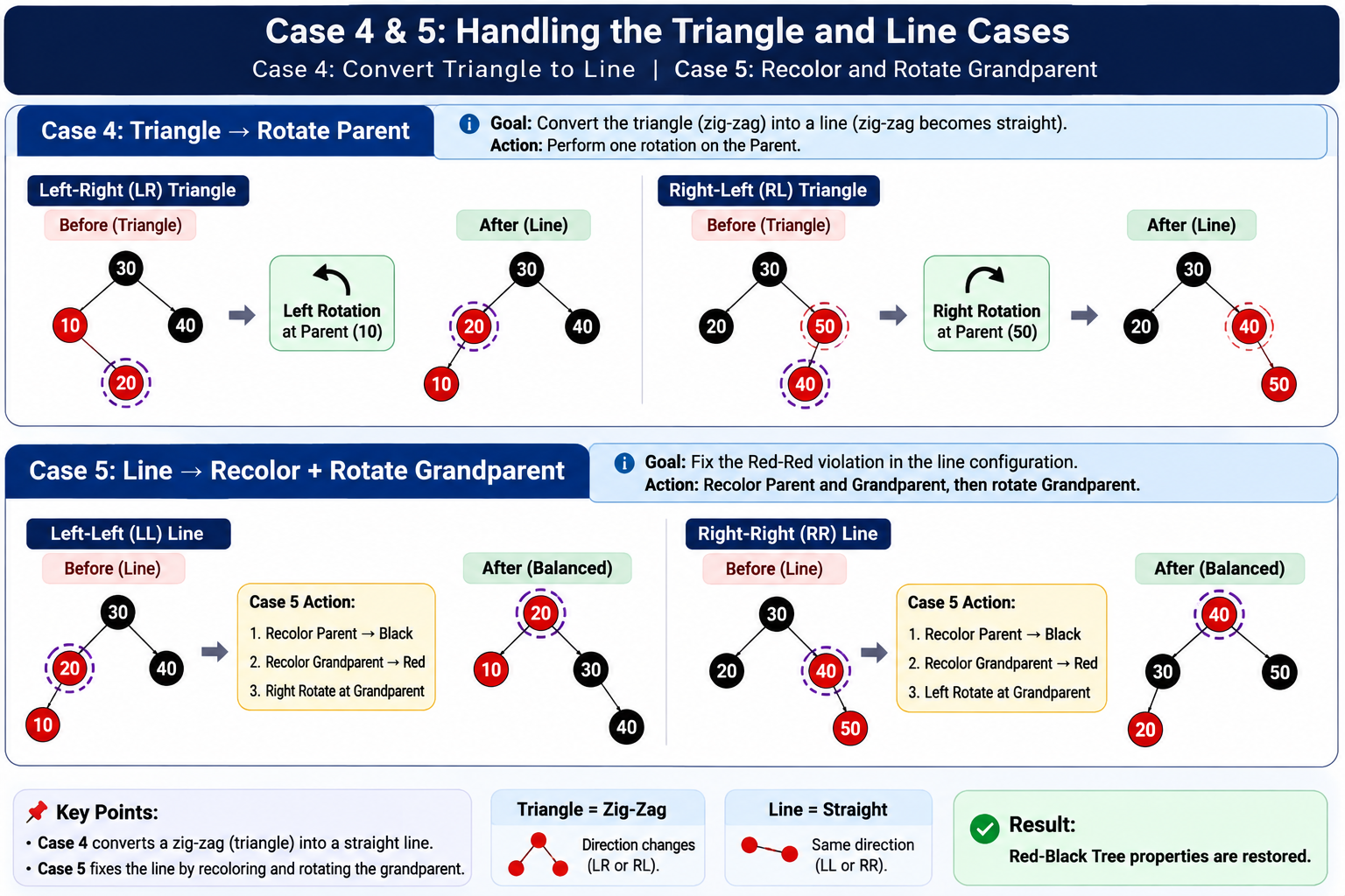
Case 4: Parent is Red, Uncle is Black (Triangle)
The "triangle" is simply a mnemonic for the zig-zag (LR or RL) configuration, while the "line" refers to the straight (LL or RR) configuration.
Suppose
- Grandparent (G)
- Parent (P)
- Newly inserted node (N)
Left-Right (LR) Triangle
         ⚫(30) G
        /
      🔴 (10) P
        \
         🔴(20)  N
Right-Left (RL) Triangle
         ⚫ 30 G
          \
           🔴 50  P
          /
        🔴 40 N
Triangle configurations are resolved by performing a rotation on the parent node, which converts the triangle into a line configuration.
flowchart LR

subgraph BEFORE["Before Insertion"]
direction TB

G(("30"))
P(("10"))
U(("40"))

G --> P
G --> U

style G fill:#222222,stroke:#000000,stroke-width:3px,color:#fff
style P fill:#E53935,stroke:#B71C1C,stroke-width:3px,color:#fff
style U fill:#222222,stroke:#000000,stroke-width:3px,color:#fff

end

A["➕ Insert 20"]

subgraph TRIANGLE["After BST Insertion (Triangle)"]
direction TB

G1(("30"))
P1(("10"))
U1(("40"))
N(("20"))

G1 --> P1
G1 --> U1
P1 --> N

style G1 fill:#222222,stroke:#000000,stroke-width:3px,color:#fff
style P1 fill:#E53935,stroke:#B71C1C,stroke-width:3px,color:#fff
style U1 fill:#222222,stroke:#000000,stroke-width:3px,color:#fff

%% Newly inserted node
style N fill:#E53935,stroke:#7C3AED,stroke-width:4px,stroke-dasharray:8 4,color:#fff

end

R["🔄 Left Rotation<br/>at Parent (10)"]

subgraph AFTER["Triangle becomes Line (Case 5)"]
direction TB

G2(("30"))
N2(("20"))
U2(("40"))
P2(("10"))

G2 --> N2
G2 --> U2
N2 --> P2

style G2 fill:#222222,stroke:#000000,stroke-width:3px,color:#fff
style U2 fill:#222222,stroke:#000000,stroke-width:3px,color:#fff
style P2 fill:#E53935,stroke:#B71C1C,stroke-width:3px,color:#fff

%% Inserted node
style N2 fill:#E53935,stroke:#7C3AED,stroke-width:4px,stroke-dasharray:8 4,color:#fff

end

BEFORE --> A --> TRIANGLE --> R --> AFTER

linkStyle default stroke:#64748B,stroke-width:2px
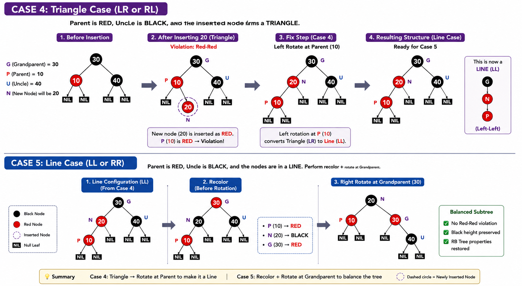
Case 5: Parent is Red, Uncle is Black (Line)
After Case 4 converts the triangle into a line, Case 5 performs:
Recolor Parent → ⚫ Black Grandparent → 🔴 Red Rotate the Grandparent
For the Left-Left (LL) configuration:
flowchart LR

subgraph BEFORE["Line Configuration (After Case 4)"]
direction TB

G(("30"))
N(("20"))
U(("40"))
P(("10"))

G --> N
G --> U
N --> P

%% Grandparent
style G fill:#222222,stroke:#000000,stroke-width:3px,color:#fff

%% Parent (Inserted node from Case 4)
style N fill:#E53935,stroke:#7C3AED,stroke-width:4px,stroke-dasharray:8 4,color:#fff

%% Child
style P fill:#E53935,stroke:#B71C1C,stroke-width:3px,color:#fff

%% Uncle
style U fill:#222222,stroke:#000000,stroke-width:3px,color:#fff

end

R["🎨 Recolor<br/>🔄 Right Rotation<br/>at Grandparent (30)"]

subgraph AFTER["Balanced Tree"]
direction TB

N2(("20"))
P2(("10"))
G2(("30"))
U2(("40"))

N2 --> P2
N2 --> G2
G2 --> U2

%% New Root of Subtree
style N2 fill:#222222,stroke:#7C3AED,stroke-width:4px,stroke-dasharray:8 4,color:#fff

%% Grandparent becomes Red
style G2 fill:#E53935,stroke:#B71C1C,stroke-width:3px,color:#fff

%% Child
style P2 fill:#E53935,stroke:#B71C1C,stroke-width:3px,color:#fff

%% Uncle
style U2 fill:#222222,stroke:#000000,stroke-width:3px,color:#fff

end

BEFORE --> R --> AFTER

linkStyle default stroke:#64748B,stroke-width:2px
Insert Time Complexity in Red-Black Tree
| Operation | Complexity |
|---|---|
| BST Insertion | |
| Recoloring | |
| Rotation | |
| Overall Insertion |
Because a Red-Black Tree guarantees its height is bounded by
All fundamental operations take O(log n) time in the worst case.
Red-Black Tree Properties
| Operation | Average | Worst | Explanation |
|---|---|---|---|
| Search | Traverse from root to leaf. | ||
| Insert | BST insertion followed by recoloring and at most two rotations. | ||
| Delete | BST deletion followed by rebalancing and recoloring. | ||
| Find Minimum | Follow the leftmost path. | ||
| Find Maximum | Follow the rightmost path. | ||
| Successor / Predecessor | Search along one root-to-leaf path. | ||
| Rotation | Only a few pointers are updated. | ||
| Recoloring | Only node colors change. |
Red-Black Tree vs AVL Trade-off
| Feature | AVL Tree | Red-Black Tree |
|---|---|---|
| Search Performance | ⭐ Faster | Slightly slower |
| Insert Performance | Slower | ⭐ Faster |
| Delete Performance | Slower | ⭐ Faster |
| Height | Smaller | Larger |
| Rotations | More frequent | Less frequent |
| Complexity | Moderate | Higher |
BST Limitations
While a BST works efficiently in RAM by minimizing element comparisons, a disk-based system is bottlenecked by the number of separate disk block reads (disk I/O operations) required to traverse deep tree structures
These operations are slow so a deep tree is a performance bottleneck.
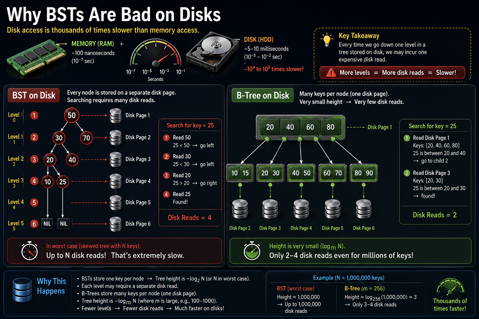
B-Trees are designed to minimize disk I/O by keeping the tree height low and storing multiple keys in each node.
B-TREE
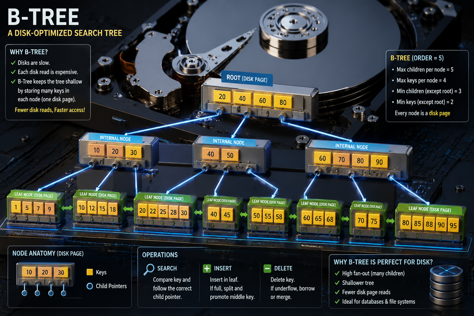
A self-balancing multi-way search tree optimized for disks, SSDs, and databases.
Unlike AVL and Red-Black Trees, a B-Tree stores multiple keys in a single node, drastically reducing the tree height and minimizing expensive disk accesses.
Node Structure
- Each node contains multiple keys and child pointers.
- Keys are stored in sorted order.
Order of b-tree
Maximum number of children a node can have is called the order of the B-Tree.
flowchart TB

    subgraph NODE["B-Tree Node (Order = 4)"]
    direction TB

    K["Keys (Sorted)<br/>10 | 25 | 40"]

    P["Child Pointers<br/>P0 | P1 | P2 | P3"]

    K --> P
    end

    P --> R0["P0 : Keys < 10"]
    P --> R1["P1 : 10 ≤ Keys < 25"]
    P --> R2["P2 : 25 ≤ Keys < 40"]
    P --> R3["P3 : Keys ≥ 40"]

    style K fill:#10B981,stroke:#047857,stroke-width:2px,color:#fff
    style P fill:#3B82F6,stroke:#1D4ED8,stroke-width:2px,color:#fff

    style R0 fill:#F59E0B,stroke:#B45309,color:#fff
    style R1 fill:#F59E0B,stroke:#B45309,color:#fff
    style R2 fill:#F59E0B,stroke:#B45309,color:#fff
    style R3 fill:#F59E0B,stroke:#B45309,color:#fff

    linkStyle default stroke:#64748B,stroke-width:2px
General Formula
| Property | Formula |
|---|---|
| Order | |
| Maximum Children per Node | |
| Maximum Keys | |
| Minimum Children (non-root) | |
| Minimum Keys (non-root) |
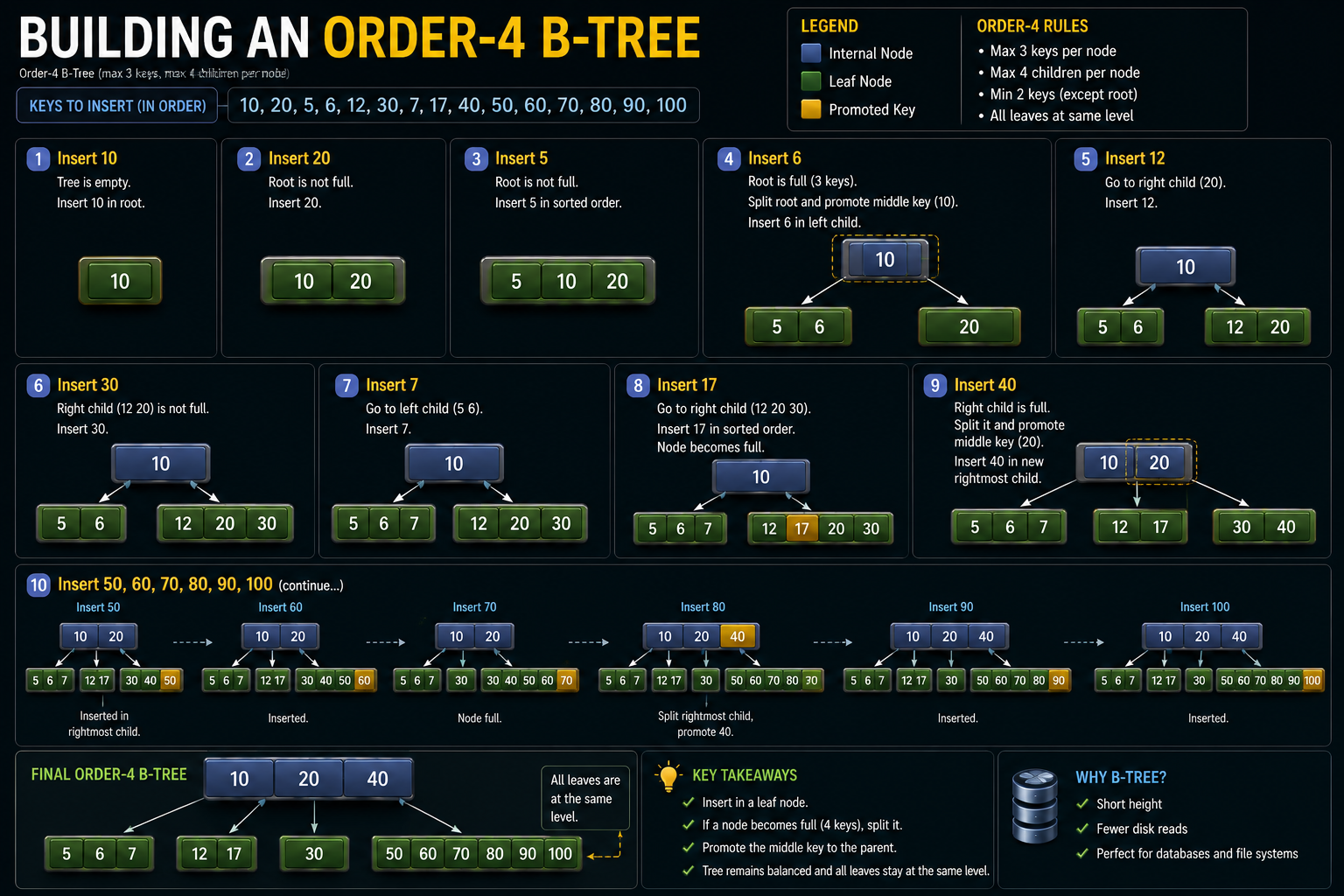
Insertion in B-Tree
- Search for the correct leaf node.
- If the leaf has room, insert the key in sorted order.
- If the leaf is full:
- Split the node.
- Promote the middle key to the parent.
- If the parent becomes full, repeat the split upward.
- If the root splits, create a new root.
B-Tree Operations
| Operation | Complexity |
|---|---|
| Search | O(log n) |
| Insert | O(log n) |
| Delete | O(log n) |
| Split | O(1) |
| Merge | O(1) |
✅ B-Tree Advantages
- Extremely short trees
- Disk optimized
- Few page reads
- Excellent for large datasets
- Efficient insert/delete
- Balanced automatically
❌ B-Tree Limitations
- More complex implementation
- Higher memory overhead per node
- Less efficient for tiny in-memory datasets
- Node splitting and merging add implementation complexity
Applications
- SQL databases (MySQL, PostgreSQL, SQLite)
- Filesystems (NTFS, HFS+, ext4, APFS)
- Key-value stores
- SSD and HDD indexes
- Database indexes
- Large-scale storage engines
AVL vs Red-Black vs B-Tree
| Feature | AVL | Red-Black | B-Tree |
|---|---|---|---|
| Children per node | 2 | 2 | Many |
| Height | Smallest | Slightly taller | Much smaller |
| Disk Friendly | ❌ | ❌ | ✅ |
| Memory | RAM | RAM | Disk/RAM |
| Databases | ❌ | Rare | ✅ |
| Filesystems | ❌ | Rare | ✅ |
B Tree limitations
B-Trees work well for storage
But databases frequently perform
- Range queries
- Ordered scans
- Index traversal
Instead of repeatedly climbing the tree,
B+ Trees allow walking on leafs using linked leaves.
B+ Tree
A B+ Tree is a variation of a B-Tree that stores all values in the leaf nodes and maintains a linked list of leaves for efficient range queries.
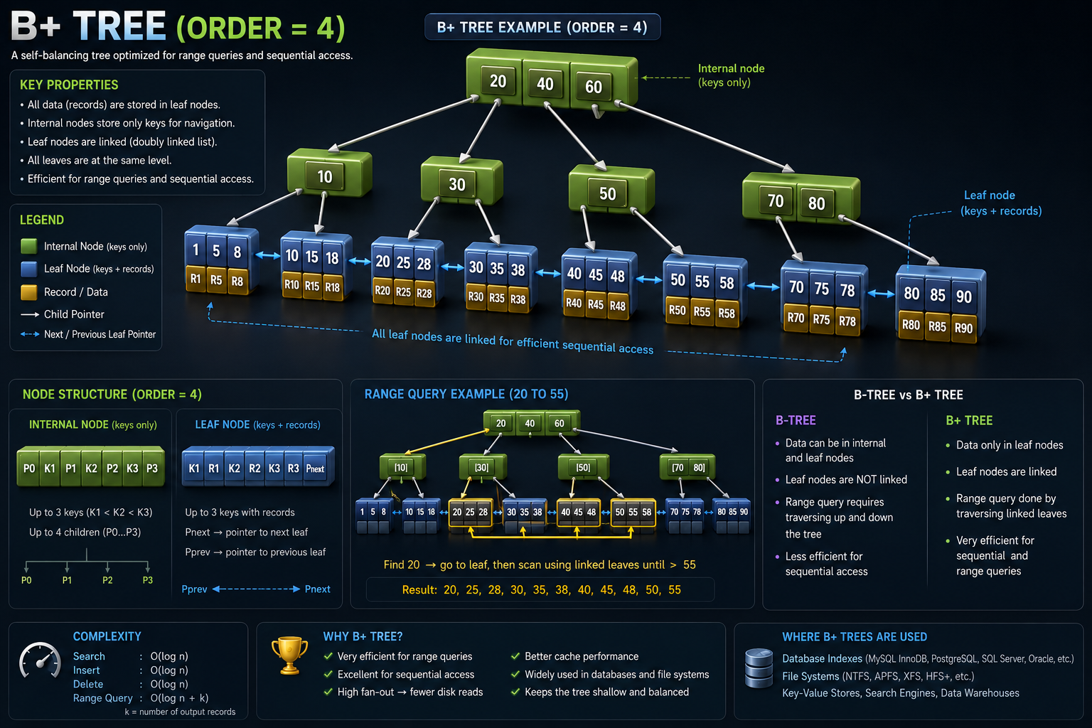
flowchart TB

%% Root
R["20 | 40 | 60"]

%% Internal Nodes
I1["10"]
I2["30"]
I3["50"]
I4["70 | 80"]

R --> I1
R --> I2
R --> I3
R --> I4

%% Leaf Nodes
L1["1 | 5 | 8<br/>R1 R5 R8"]
L2["10 | 15 | 18<br/>R10 R15 R18"]
L3["20 | 25 | 28<br/>R20 R25 R28"]
L4["30 | 35 | 38<br/>R30 R35 R38"]
L5["40 | 45 | 48<br/>R40 R45 R48"]
L6["50 | 55 | 58<br/>R50 R55 R58"]
L7["70 | 75 | 78<br/>R70 R75 R78"]
L8["80 | 85 | 90<br/>R80 R85 R90"]

I1 --> L1
I1 --> L2

I2 --> L3
I2 --> L4

I3 --> L5
I3 --> L6

I4 --> L7
I4 --> L8

%% Linked Leaves
L1 -.-> L2
L2 -.-> L3
L3 -.-> L4
L4 -.-> L5
L5 -.-> L6
L6 -.-> L7
L7 -.-> L8

%% Styles
style R fill:#10B981,stroke:#047857,stroke-width:3px,color:#fff

style I1 fill:#10B981,stroke:#047857,stroke-width:2px,color:#fff
style I2 fill:#10B981,stroke:#047857,stroke-width:2px,color:#fff
style I3 fill:#10B981,stroke:#047857,stroke-width:2px,color:#fff
style I4 fill:#10B981,stroke:#047857,stroke-width:2px,color:#fff

style L1 fill:#3B82F6,stroke:#1D4ED8,stroke-width:2px,color:#fff
style L2 fill:#3B82F6,stroke:#1D4ED8,stroke-width:2px,color:#fff
style L3 fill:#3B82F6,stroke:#1D4ED8,stroke-width:2px,color:#fff
style L4 fill:#3B82F6,stroke:#1D4ED8,stroke-width:2px,color:#fff
style L5 fill:#3B82F6,stroke:#1D4ED8,stroke-width:2px,color:#fff
style L6 fill:#3B82F6,stroke:#1D4ED8,stroke-width:2px,color:#fff
style L7 fill:#3B82F6,stroke:#1D4ED8,stroke-width:2px,color:#fff
style L8 fill:#3B82F6,stroke:#1D4ED8,stroke-width:2px,color:#fff

%% Child pointers
linkStyle 0,1,2,3,4,5,6,7,8,9,10,11 stroke:#64748B,stroke-width:2px

%% Leaf links
linkStyle 12,13,14,15,16,17,18 stroke:#2563EB,stroke-width:2px,stroke-dasharray:5 5
Range Queries
WHERE Age BETWEEN 20 AND 40
B-Tree vs B+ Tree
| Feature | B-Tree | B+ Tree |
|---|---|---|
| Internal nodes store data | ✅ Yes | ❌ No |
| Leaf nodes store data | ✅ Yes | ✅ Yes |
| Leaf nodes linked | ❌ | ✅ |
| Range queries | Good | ⭐ Excellent |
| Sequential scan | Moderate | ⭐ Excellent |
| Database usage | Rare | ⭐ Very Common |
B+ Tree Complexity
| Operation | Complexity |
|---|---|
| Search | |
| Insert | |
| Delete | |
| Range Query |
where k = number of matching records.
✅ B+ Tree Advantages
- Extremely efficient range scans
- Sequential traversal
- Small internal nodes
- High fan-out
- Few disk reads
- Better cache performance
- Excellent for databases
❌ B+ Tree Limitations
- More complex implementation
- Higher memory overhead per node
- Less efficient for tiny in-memory datasets
- Node splitting and merging add implementation complexity
#️⃣ Hash Table
A data structure that stores
key-valuepairs and uses a hash function to achieve near constant-time lookups.
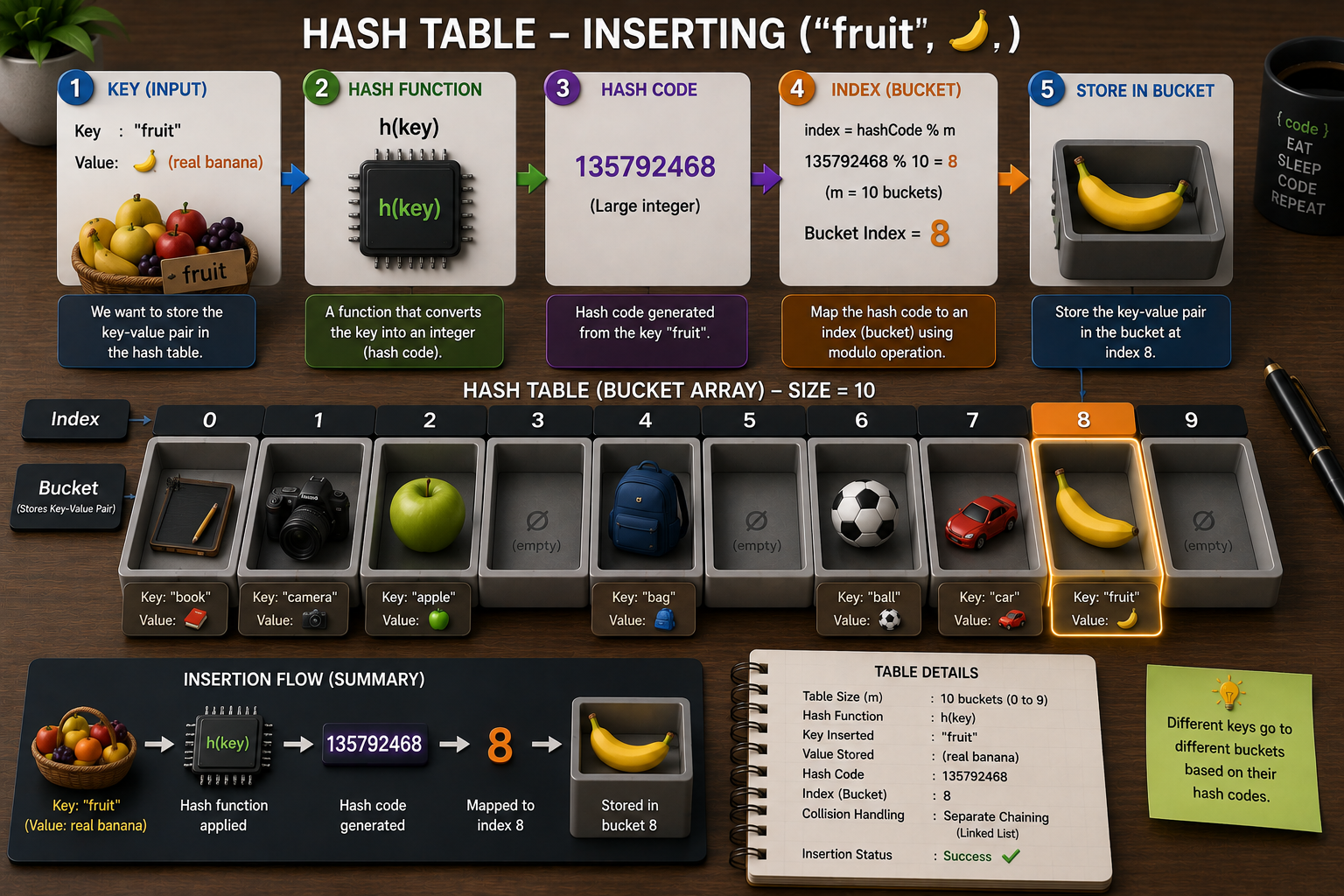
A hash table uses a hash function to compute an index, also called a hash code, into an array of buckets or slots, from which the desired value can be found.
Hash code is generated by a hash function that takes a key and returns an integer.
hash("fruit") = 135792468
hashcode is then mapped to an index in the hash table using the modulo operator with the size of the table.
index = 135792468 % 10 = 8
Store banana in index 8 of the hash table.
 ️
️
Lookup in Hash Table
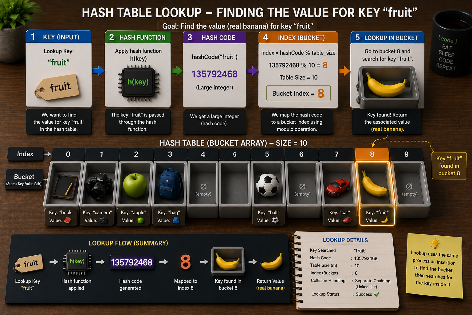
During lookup, the key is hashed and the resulting hash indicates where the corresponding value is stored.
A map implemented by a hash table is called a hash map.
Hash Collisions
Explain
hash("cat") = 4 hash("dog") = 4
Both map to the same bucket
Open Addressing
Open Addressing is a collision resolution technique where all key-value pairs are stored directly inside the hash table. If a bucket is occupied, the algorithm probes other buckets until it finds an empty slot.
- Compute the hash code.
- Find the target bucket.
- If the bucket is empty, insert the key.
- If the bucket is occupied, probe another bucket.
- Repeat until an empty bucket is found.
There are three common probing strategies:
1. Linear Probing
Check the next bucket until an empty one is found.
where
- = hash value
- = probe number (0,1,2,...)
- = table size
Example: Hash = 5
Bucket 5 occupied --> Try 6(+1) --> Try 7(+2) --> Insert
2. Quadratic Probing
Check buckets at positions determined by a quadratic function.
where
- = hash value
- = probe number (0,1,2,...)
- = constants
Example: Hash = 5
Bucket 5 occupied --> Try 6 (+1²) --> Try 9 (+2²) --> Try 14 (+3²)
3. Double Hashing
Use a second hash function to determine the step size for probing.
Double hashing provides the best distribution.
where
- = first hash function
- = second hash function
- = probe number (0,1,2,...)
- = table size
Load Factor
The Load Factor measures how full a hash table is.
It is the ratio of the number of stored key-value pairs to the total number of buckets.
Where:
- α = Load Factor
- n = Number of stored key-value pairs
- m = Number of buckets
As the load factor increases:
- More buckets become occupied.
- More collisions occur.
- More probing or chaining is required.
- Search and insertion become slower.
Rehashing
When the load factor exceeds a threshold (commonly 0.75), the hash table grows.
Example
Buckets = 10
Elements = 8
Load Factor = 0.8
Resize the table to 20 buckets and rehash all existing elements.
Buckets = 20
Elements = 8
Load Factor = 0.4
Collisions decrease, restoring near O(1) performance.
Hash Table Usage
Use a Hash Table when:
- You need fast key-based lookup.
- Data does not need to be sorted.
- Range queries are not required.
- Average-case performance matters most.
Avoid a Hash Table when:
- You need sorted iteration.
- You need range queries (use a B+ Tree or balanced BST).
- You need to find the minimum or maximum key efficiently.
Operations
| Operation | Average | Worst |
|---|---|---|
| Search | O(1) | O(n) |
| Insert | O(1) | O(n) |
| Delete | O(1) | O(n) |
Advantages
- Extremely fast lookups
- Simple implementation
- Excellent for caches
- Great average performance
Limitations
- No ordering
- No range queries
- Depends on good hash function
- Rehashing can be expensive
- Worst-case O(n)
Hash Table Limitations vs Trie
Hash tables are excellent for exact lookups but fail for prefix searches, autocomplete, and ordered traversals.
Hash table can tell if banana exists, but cannot tell if any words start with
- "ban"
- "bana"
- "banan"
Existing words cannot be traversed in order.
Trie solves these problems by storing words in a tree structure, allowing for efficient prefix searches and ordered traversals.
Trie (Prefix Tree)
A Trie is a tree-based data structure that stores strings one character at a time, enabling extremely fast prefix searches, autocomplete, and dictionary lookups.
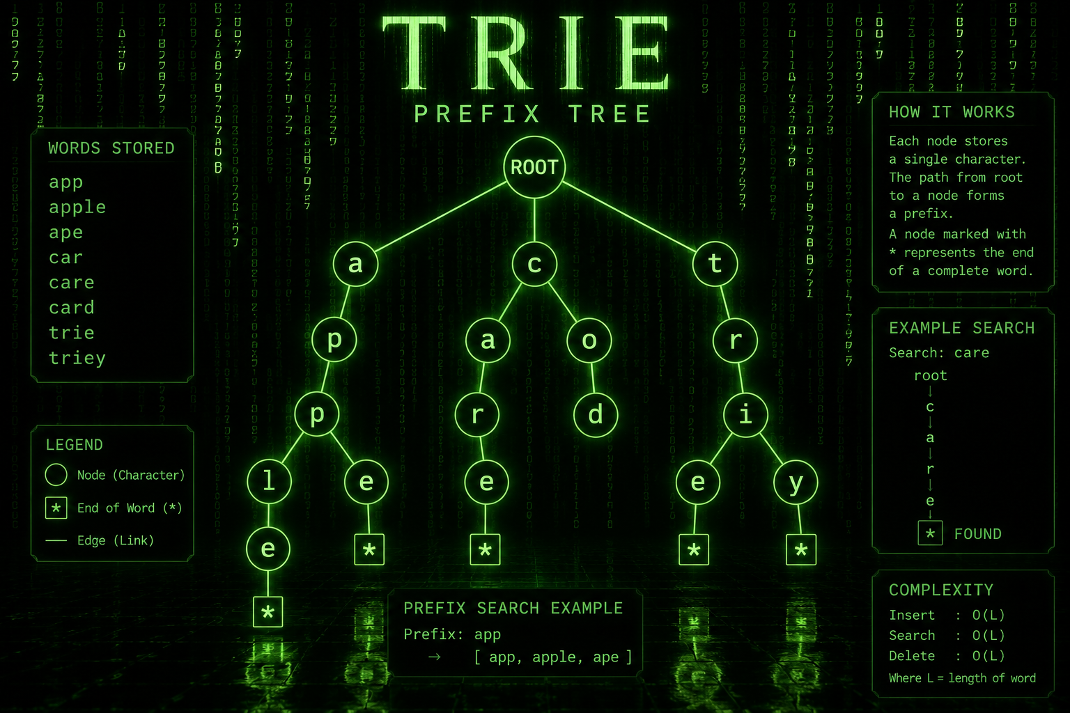
Trie efficiently solve
- Prefix search
- Autocomplete
- Spell checking
- Dictionary lookup
without scanning every word.
Trie vs Hash Table
| Feature | Trie | Hash Table |
|---|---|---|
| Exact Search | O(L) | ⭐ Average O(1) |
| Prefix Search | ⭐ Excellent | ❌ Not Supported |
| Autocomplete | ⭐ Excellent | ❌ |
| Lexicographical Order | ✅ Yes | ❌ No |
| Memory Usage | High | Low |
| Cache Locality | Poor | Good |
| Ordered Traversal | ✅ Yes | ❌ |
Trie Node Structure
Every Trie node typically contains three components:
- Character
- End-of-Word Flag
- Child References
                TrieNode
        ┌────────────────────────┐
        │ Character : 'a'        │
        ├────────────────────────┤
        │ isWord   : false       │
        ├────────────────────────┤
        │ Children               │
        │  ├── 'p' → TrieNode    │
        │  ├── 'b' → TrieNode    │
        │  ├── 'c' → TrieNode    │
        │  └── ...               │
        └────────────────────────┘
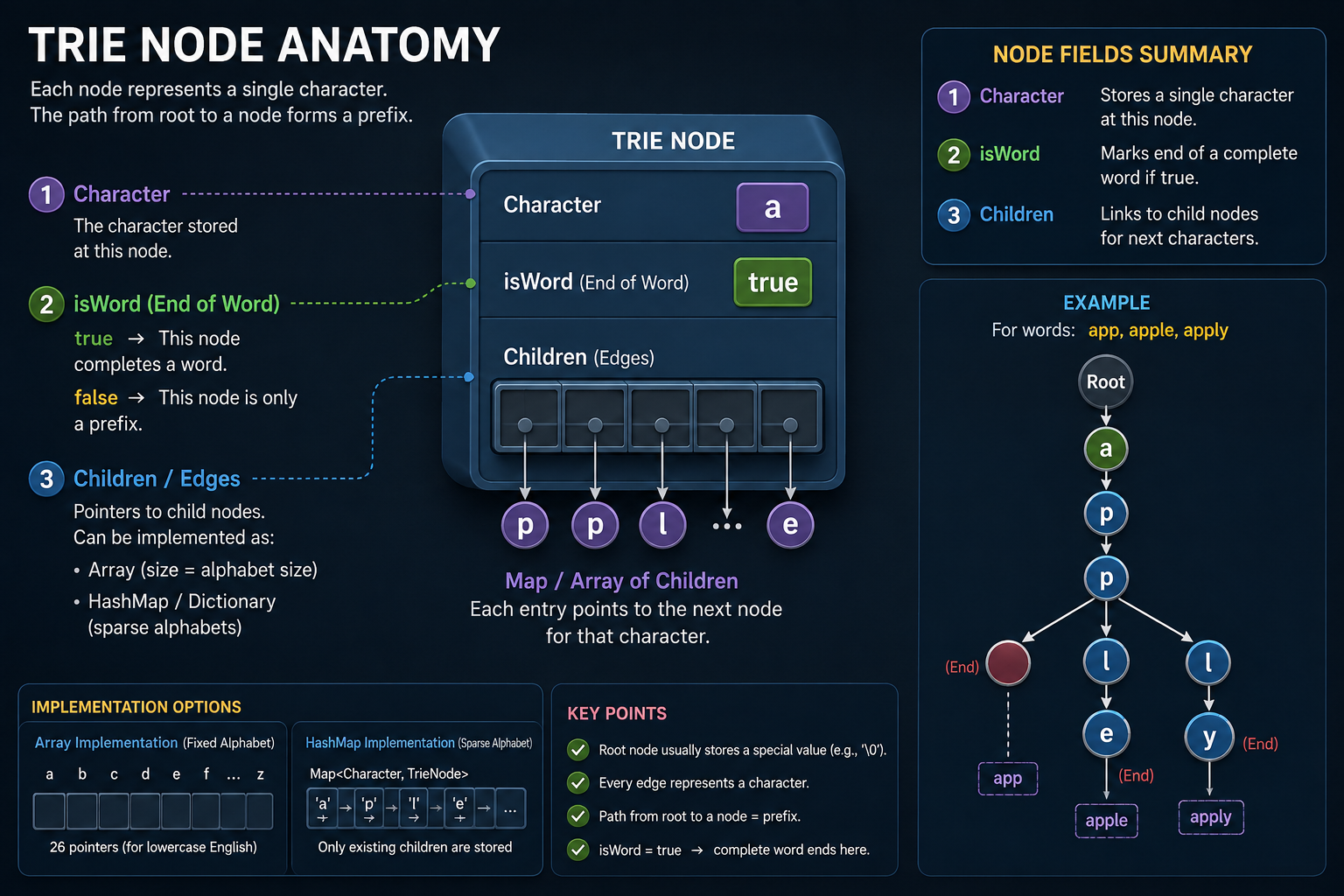
Unlike a Binary Tree node, which has only left and right pointers, a Trie node can have many children, one for each possible next character.
Words represented
- card
- care
- cart
- dog
flowchart TB

    ROOT(("Root"))

    ROOT --> C(("c"))
    C --> A(("a"))
    A --> R(("r"))

    %% Shared Prefix
    R --> D(("d"))
    R --> E(("e"))
    R --> T(("t"))

    D --> END1(("✓"))
    E --> END2(("✓"))
    T --> END3(("✓"))

    %% Another Branch
    ROOT --> D1(("d"))
    D1 --> O(("o"))
    O --> G(("g"))
    G --> END4(("✓"))

    %% Shared Prefix
    style ROOT fill:#10B981,stroke:#047857,stroke-width:3px,color:#fff
    style C fill:#10B981,stroke:#047857,stroke-width:3px,color:#fff
    style A fill:#10B981,stroke:#047857,stroke-width:3px,color:#fff
    style R fill:#10B981,stroke:#047857,stroke-width:3px,color:#fff

    %% Unique Suffixes
    style D fill:#3B82F6,stroke:#1D4ED8,stroke-width:2px,color:#fff
    style E fill:#3B82F6,stroke:#1D4ED8,stroke-width:2px,color:#fff
    style T fill:#3B82F6,stroke:#1D4ED8,stroke-width:2px,color:#fff

    style D1 fill:#3B82F6,stroke:#1D4ED8,stroke-width:2px,color:#fff
    style O fill:#3B82F6,stroke:#1D4ED8,stroke-width:2px,color:#fff
    style G fill:#3B82F6,stroke:#1D4ED8,stroke-width:2px,color:#fff

    %% End of Word
    style END1 fill:#F59E0B,stroke:#B45309,stroke-width:2px,color:#fff
    style END2 fill:#F59E0B,stroke:#B45309,stroke-width:2px,color:#fff
    style END3 fill:#F59E0B,stroke:#B45309,stroke-width:2px,color:#fff
    style END4 fill:#F59E0B,stroke:#B45309,stroke-width:2px,color:#fff

    linkStyle default stroke:#64748B,stroke-width:2px
Operations
The algorithm never scans the entire dictionary.
Instead, it follows exactly one path.
This is why Trie operations depend on word length, not on the number of stored words.
| Operation | Complexity |
|---|---|
| Search | |
| Insert | |
| Delete | |
| Prefix Search | |
| Autocomplete |
Where
- : Length of the input word or prefix
- : Number of words returned during autocomplete
Usage
- Real-World Applications
- Google Search
- IDE Autocomplete
- Mobile Keyboard
- Spell Checker
Related Posts
- 🧱 Data Structures — linear structures (arrays, linked lists, stacks, queues) these trees and graphs build on
- 🔢 Algorithmic Complexity — the Big O notation used throughout every table above
- 🔎 Searching Algorithms — Balanced BST search is the tree-based search case worked through here
- 🗄️ Database Comparison — B-Trees index relational databases; hash tables back key-value stores; graphs back graph databases