🕸️ Graph Data Structures: Adjacency List vs Matrix, BFS & DFS
Graphs from the ground up — vertices and edges, why there's no single Big O for a graph, adjacency list vs adjacency matrix tradeoffs, and why BFS and DFS traversal cost is the foundation every graph algorithm builds on.
🌲 Trees Deep Dive: BST, AVL Rotations, Red-Black Trees, B-Trees & B+ Trees
🔢 Algorithmic Complexity: Big O From First Principles
🕸️ Graph
A graph is a collection of vertices (nodes) connected by edges.
Mathematically,
where
🎱 Vertices :
A vertex (or node) represents an object in the graph.
Adjacent Vertices (Neighbors)
Two vertices are adjacent if they are connected by an edge.
Path
A path is a sequence of vertices where each adjacent pair is connected by an edge.
Simple Path
A simple path is a path that does not contain any repeated vertices.
Cycle
A cycle is a path that starts and ends at the same vertex, with no other repeated vertices.
Self Loop
An edge that connects a vertex to itself.
Connected Component
A connected component is a group of vertices connected to each other.
A connected component is a subgraph in which any two vertices are connected to each other by paths and which is connected to no additional vertices in the supergraph.
🪈 Edge :
An edge represents a relationship between two vertices.
Example:
- Road
- Flight
- Network Cable
- Friendship
Weight
A weighted graph is a graph in which each edge has a numerical value (weight) associated with it.
Example:
- Distance
- Cost
- Time
- Bandwidth
- Probability
Degree
The degree of a vertex is the number of edges connected to it.
Degree is number of connections a vertex has.
In a directed graph, we have in-degree and out-degree.
In-Degree (Directed Graph)
The in-degree of a vertex is the number of edges coming into it.
Out-Degree (Directed Graph)
The out-degree of a vertex is the number of edges going out of it.
Graph Types
Graph have many types, each with its own characteristics and use cases.
Common types of graphs
| Type | Description | Example |
|---|---|---|
| Undirected Graph | A graph where edges have no direction | Friendship |
| Directed Graph | A graph where edges have a direction | Twitter follow |
| Weighted Graph | A graph where edges have weights | Road distance |
| Unweighted Graph | A graph where edges have no weights | Social network |
| Cyclic Graph | Graph contains cycles | Road network |
| Acyclic Graph | Graph contains no cycles | Family tree |
| Disconnected Graph | A graph where not all vertices are connected | Road network |
| Connected Graph | A graph where all vertices are connected | Road network |
| Sparse Graph | Few edges compared to vertices | Road network |
| Dense Graph | Many edges compared to vertices | Social network |
| Complete Graph | Every pair of vertices is connected by an edge | Social network |
| Tree | Acyclic connected graph | File system |
| Forest | Collection of trees | Multiple file systems |
More Advanced Graph Types
| Type | Description | Example |
|---|---|---|
| Bipartite | Vertices can be divided into two disjoint sets | Job assignment |
| Planar Graph | Can be drawn on a plane without edges crossing | Map of countries |
| Non-Planar Graph | Cannot be drawn on a plane without edges crossing | K5, K3,3 |
Undirected, Unweighted, Disconnected Graph Example
graph LR

    A((A))
    B((B))
    C((C))
    D((D))
    E((E))
    F((F))

    A --- B
    A --- C
    B --- D
    C --- D
    C --- E
    D --- F
    D --- E

    style A fill:#3B82F6,stroke:#1D4ED8,stroke-width:3px,color:#fff
    style B fill:#10B981,stroke:#047857,stroke-width:3px,color:#fff
    style C fill:#F59E0B,stroke:#B45309,stroke-width:3px,color:#fff
    style D fill:#EF4444,stroke:#B91C1C,stroke-width:3px,color:#fff
    style E fill:#8B5CF6,stroke:#6D28D9,stroke-width:3px,color:#fff
    style F fill:#06B6D4,stroke:#0E7490,stroke-width:3px,color:#fff

    linkStyle default stroke:#64748B,stroke-width:3px
Directed Graph
- Every edge has a direction
- Relationships are one-way
- Reverse edges must be added explicitly
graph LR

    A((A))
    B((B))
    C((C))
    D((D))
    E((E))
    F((F))

    A ---> B
    A ---> C
    B ---> D
    C ---> D
    C ---> E
    D ---> F
    D ---> E

    style A fill:#3B82F6,stroke:#1D4ED8,stroke-width:3px,color:#fff
    style B fill:#10B981,stroke:#047857,stroke-width:3px,color:#fff
    style C fill:#F59E0B,stroke:#B45309,stroke-width:3px,color:#fff
    style D fill:#EF4444,stroke:#B91C1C,stroke-width:3px,color:#fff
    style E fill:#8B5CF6,stroke:#6D28D9,stroke-width:3px,color:#fff
    style F fill:#06B6D4,stroke:#0E7490,stroke-width:3px,color:#fff

    linkStyle default stroke:#64748B,stroke-width:3px
Weighted Graph
graph LR

    A((A))
    B((B))
    C((C))
    D((D))
    E((E))
    F((F))

    A ---|4| B
    A ---|2| C
    B ---|5| D
    C ---|1| D
    C ---|7| E
    D ---|6| F
    D ---|3| E

    style A fill:#3B82F6,stroke:#1D4ED8,stroke-width:3px,color:#fff
    style B fill:#10B981,stroke:#047857,stroke-width:3px,color:#fff
    style C fill:#F59E0B,stroke:#B45309,stroke-width:3px,color:#fff
    style D fill:#EF4444,stroke:#B91C1C,stroke-width:3px,color:#fff
    style E fill:#8B5CF6,stroke:#6D28D9,stroke-width:3px,color:#fff
    style F fill:#06B6D4,stroke:#0E7490,stroke-width:3px,color:#fff

    linkStyle default stroke:#64748B,stroke-width:3px
Cyclic Graph
graph LR

    A((A))
    B((B))
    C((C))
    D((D))
    E((E))
    F((F))

    A --- B
    A --- C
    B --- D
    C --- D
    C --- E
    D --- E
    D --- F
    E --- F

    style A fill:#3B82F6,stroke:#1D4ED8,stroke-width:3px,color:#fff
    style B fill:#10B981,stroke:#047857,stroke-width:3px,color:#fff
    style C fill:#F59E0B,stroke:#B45309,stroke-width:3px,color:#fff
    style D fill:#EF4444,stroke:#B91C1C,stroke-width:3px,color:#fff
    style E fill:#8B5CF6,stroke:#6D28D9,stroke-width:3px,color:#fff
    style F fill:#06B6D4,stroke:#0E7490,stroke-width:3px,color:#fff

    %% Highlight Cycle: A → B → D → C → A
    linkStyle 0 stroke:#DC2626,stroke-width:5px
    linkStyle 2 stroke:#DC2626,stroke-width:5px
    linkStyle 3 stroke:#DC2626,stroke-width:5px
    linkStyle 1 stroke:#DC2626,stroke-width:5px

    %% Remaining edges
    linkStyle 4 stroke:#64748B,stroke-width:3px
    linkStyle 5 stroke:#64748B,stroke-width:3px
    linkStyle 6 stroke:#64748B,stroke-width:3px
    linkStyle 7 stroke:#64748B,stroke-width:3px
Acyclic Graph
graph LR

    A((A))
    B((B))
    C((C))
    D((D))
    E((E))
    F((F))

    A --- B
    A --- C
    B --- D
    C --- E
    D --- F
    D --- E

    style A fill:#3B82F6,stroke:#1D4ED8,stroke-width:3px,color:#fff
    style B fill:#10B981,stroke:#047857,stroke-width:3px,color:#fff
    style C fill:#F59E0B,stroke:#B45309,stroke-width:3px,color:#fff
    style D fill:#EF4444,stroke:#B91C1C,stroke-width:3px,color:#fff
    style E fill:#8B5CF6,stroke:#6D28D9,stroke-width:3px,color:#fff
    style F fill:#06B6D4,stroke:#0E7490,stroke-width:3px,color:#fff

    linkStyle default stroke:#64748B,stroke-width:3px
Connected Graph
- Every vertex is reachable from every other vertex.
- The graph consists of a single connected component.
- There are no isolated vertices.
A connected graph may be cyclic or acyclic.
graph LR

    A((A))
    B((B))
    C((C))
    D((D))
    E((E))
    F((F))

    A --- B
    A --- C
    B --- D
    C --- E
    D --- E
    E --- F

    style A fill:#3B82F6,stroke:#1D4ED8,stroke-width:3px,color:#fff
    style B fill:#10B981,stroke:#047857,stroke-width:3px,color:#fff
    style C fill:#F59E0B,stroke:#B45309,stroke-width:3px,color:#fff
    style D fill:#EF4444,stroke:#B91C1C,stroke-width:3px,color:#fff
    style E fill:#8B5CF6,stroke:#6D28D9,stroke-width:3px,color:#fff
    style F fill:#06B6D4,stroke:#0E7490,stroke-width:3px,color:#fff

    linkStyle default stroke:#64748B,stroke-width:3px
Tree
A tree is a special type of graph that is connected and contains no cycles.
- Connected
- No cycles : exactly one simple path between any two vertices
- Every edge is a bridge : removing any edge disconnects the graph
For vertices, a tree always has edges
graph TD

    A((A))
    B((B))
    C((C))
    D((D))
    E((E))
    F((F))
    G((G))

    A --- B
    A --- C
    B --- D
    B --- E
    C --- F
    C --- G

    style A fill:#3B82F6,stroke:#1D4ED8,stroke-width:3px,color:#fff
    style B fill:#10B981,stroke:#047857,stroke-width:3px,color:#fff
    style C fill:#F59E0B,stroke:#B45309,stroke-width:3px,color:#fff
    style D fill:#EF4444,stroke:#B91C1C,stroke-width:3px,color:#fff
    style E fill:#8B5CF6,stroke:#6D28D9,stroke-width:3px,color:#fff
    style F fill:#06B6D4,stroke:#0E7490,stroke-width:3px,color:#fff
    style G fill:#F97316,stroke:#C2410C,stroke-width:3px,color:#fff

    linkStyle default stroke:#64748B,stroke-width:3px
Forest
A forest is a collection of disconnected trees.
In other words, a forest is an acyclic graph whose connected components are all trees.
- Collection of one or more trees
- No cycles
- Disconnected graph
- Every connected component is a tree
Removing an edge from a tree creates a forest
For a forest with
- vertices
- trees (connected components)
the number of edges is
graph TD

subgraph "Tree 1"
    A((A))
    B((B))
    C((C))
    D((D))

    A --- B
    A --- C
    B --- D
end

subgraph "Tree 2"
    E((E))
    F((F))
    G((G))

    E --- F
    E --- G
end

style A fill:#3B82F6,stroke:#1D4ED8,stroke-width:3px,color:#fff
style B fill:#10B981,stroke:#047857,stroke-width:3px,color:#fff
style C fill:#F59E0B,stroke:#B45309,stroke-width:3px,color:#fff
style D fill:#EF4444,stroke:#B91C1C,stroke-width:3px,color:#fff

style E fill:#8B5CF6,stroke:#6D28D9,stroke-width:3px,color:#fff
style F fill:#06B6D4,stroke:#0E7490,stroke-width:3px,color:#fff
style G fill:#F97316,stroke:#C2410C,stroke-width:3px,color:#fff

linkStyle default stroke:#64748B,stroke-width:3px
| Structure | Connected | Cycles | Components |
|---|---|---|---|
| Tree | ✅ | ❌ | 1 |
| Forest | ❌ | ❌ | ≥ 1 |
| Connected Graph | ✅ | ✅ / ❌ | 1 |
| Disconnected Graph | ❌ | ✅ / ❌ | ≥ 2 |
Directed Acyclic Graph (DAG)
A Directed Acyclic Graph (DAG) is a directed graph that contains no directed cycles.
Once you follow the direction of the edges, you can never return to the starting vertex.
- Directed graph
- No directed cycles
- One or more valid topological orderings
- Represents dependency relationships
A node depends only on its predecessors
graph TD

    A((Source))
    B((Compile))
    C((Test))
    D((Package))
    E((Deploy))
    F((Production))

    A --> B
    A --> C
    B --> D
    C --> D
    D --> E
    E --> F

    style A fill:#3B82F6,stroke:#1D4ED8,stroke-width:3px,color:#fff
    style B fill:#10B981,stroke:#047857,stroke-width:3px,color:#fff
    style C fill:#F59E0B,stroke:#B45309,stroke-width:3px,color:#fff
    style D fill:#EF4444,stroke:#B91C1C,stroke-width:3px,color:#fff
    style E fill:#8B5CF6,stroke:#6D28D9,stroke-width:3px,color:#fff
    style F fill:#06B6D4,stroke:#0E7490,stroke-width:3px,color:#fff

    linkStyle default stroke:#64748B,stroke-width:3px
Bipartite Graph
A bipartite graph is a graph whose vertices can be divided into two disjoint sets, such that every edge connects a vertex from one set to a vertex in the other.
Bipartite graphs model relationships between two different types of entities,
-
Vertices are divided into two disjoint sets
-
Every edge connects vertices from different sets
-
No edges exist within the same set
Students ─────────▶ Courses
No two vertices within the same set are directly connected.
graph LR

subgraph "Students"
    A((Alice))
    B((Bob))
    C((Charlie))
end

subgraph "Courses"
    X((AI))
    Y((Database))
    Z((Algorithms))
end

A --- X
A --- Y
B --- Y
B --- Z
C --- X
C --- Z

style A fill:#3B82F6,stroke:#1D4ED8,stroke-width:3px,color:#fff
style B fill:#10B981,stroke:#047857,stroke-width:3px,color:#fff
style C fill:#F59E0B,stroke:#B45309,stroke-width:3px,color:#fff

style X fill:#8B5CF6,stroke:#6D28D9,stroke-width:3px,color:#fff
style Y fill:#EF4444,stroke:#B91C1C,stroke-width:3px,color:#fff
style Z fill:#06B6D4,stroke:#0E7490,stroke-width:3px,color:#fff

linkStyle default stroke:#64748B,stroke-width:3px
Planar Graph
A planar graph is a graph that can be drawn on a plane such that no two edges intersect except at their endpoints.
- Can be drawn without crossing edges
- Edges intersect only at vertices
- Divides the plane into regions (faces)
Satisfies Euler's Formula
where:
- = Number of vertices
- = Number of edges
- = Number of faces (including the outer face)
graph TD

    A((A))
    B((B))
    C((C))
    D((D))
    E((E))

    A --- B
    A --- C
    B --- D
    C --- D
    B --- E
    D --- E

    style A fill:#3B82F6,stroke:#1D4ED8,stroke-width:3px,color:#fff
    style B fill:#10B981,stroke:#047857,stroke-width:3px,color:#fff
    style C fill:#F59E0B,stroke:#B45309,stroke-width:3px,color:#fff
    style D fill:#EF4444,stroke:#B91C1C,stroke-width:3px,color:#fff
    style E fill:#8B5CF6,stroke:#6D28D9,stroke-width:3px,color:#fff

    linkStyle default stroke:#64748B,stroke-width:3px
Non-Planar Graph
A non-planar graph is a graph that cannot be drawn on a plane without at least one pair of edges crossing.
No matter how you rearrange the vertices, some edges must intersect.
- Cannot be drawn without edge crossings
- At least one pair of edges must intersect
Violates planarity
graph LR

subgraph "Set U"
    A((A))
    B((B))
    C((C))
end

subgraph "Set V"
    X((X))
    Y((Y))
    Z((Z))
end

A --- X
A --- Y
A --- Z

B --- X
B --- Y
B --- Z

C --- X
C --- Y
C --- Z

style A fill:#3B82F6,stroke:#1D4ED8,stroke-width:3px,color:#fff
style B fill:#10B981,stroke:#047857,stroke-width:3px,color:#fff
style C fill:#F59E0B,stroke:#B45309,stroke-width:3px,color:#fff

style X fill:#8B5CF6,stroke:#6D28D9,stroke-width:3px,color:#fff
style Y fill:#EF4444,stroke:#B91C1C,stroke-width:3px,color:#fff
style Z fill:#06B6D4,stroke:#0E7490,stroke-width:3px,color:#fff

linkStyle default stroke:#64748B,stroke-width:3px
Planar vs Non Planar Graph
| Property | Planar | Non-Planar |
|---|---|---|
| Edge crossings required | ❌ No | ✅ Yes |
| Can be embedded in a plane | ✅ | ❌ |
| Satisfies Euler's Formula | ✅ | ❌ (in general) |
| Examples | Trees, Road Maps | , |
Sparse Graph
Loosly connected graph with few edges compared to vertices.
Most vertex pairs are not directly connected
- Typically represented using an Adjacency List
graph LR

    A((A))
    B((B))
    C((C))
    D((D))
    E((E))
    F((F))
    G((G))
    H((H))

    A --- B
    A --- C
    B --- D
    C --- E
    E --- F
    F --- G
    D --- H

    style A fill:#3B82F6,stroke:#1D4ED8,stroke-width:3px,color:#fff
    style B fill:#10B981,stroke:#047857,stroke-width:3px,color:#fff
    style C fill:#F59E0B,stroke:#B45309,stroke-width:3px,color:#fff
    style D fill:#EF4444,stroke:#B91C1C,stroke-width:3px,color:#fff
    style E fill:#8B5CF6,stroke:#6D28D9,stroke-width:3px,color:#fff
    style F fill:#06B6D4,stroke:#0E7490,stroke-width:3px,color:#fff
    style G fill:#F97316,stroke:#C2410C,stroke-width:3px,color:#fff
    style H fill:#84CC16,stroke:#4D7C0F,stroke-width:3px,color:#fff

    linkStyle default stroke:#64748B,stroke-width:3px
Dense Graph
Loosely connected graph with many edges compared to vertices.
A dense graph is a graph in which the number of edges is close to the maximum possible. Most pairs of vertices are directly connected.
graph LR

    A((A))
    B((B))
    C((C))
    D((D))
    E((E))
    F((F))

    A --- B
    A --- C
    A --- D
    A --- E

    B --- C
    B --- D
    B --- E
    B --- F

    C --- D
    C --- E
    C --- F

    D --- E
    D --- F

    E --- F

    style A fill:#3B82F6,stroke:#1D4ED8,stroke-width:3px,color:#fff
    style B fill:#10B981,stroke:#047857,stroke-width:3px,color:#fff
    style C fill:#F59E0B,stroke:#B45309,stroke-width:3px,color:#fff
    style D fill:#EF4444,stroke:#B91C1C,stroke-width:3px,color:#fff
    style E fill:#8B5CF6,stroke:#6D28D9,stroke-width:3px,color:#fff
    style F fill:#06B6D4,stroke:#0E7490,stroke-width:3px,color:#fff

    linkStyle default stroke:#64748B,stroke-width:3px
Complete Graph ()
A complete graph is a graph in which every pair of distinct vertices is connected by an edge.
- Every vertex is directly connected to every other vertex.
- Only one hop is needed to reach any vertex.
- Maximum number of edges for a graph with n vertices.
Number of Edges in a Complete Graph:
Undirected complete graph (without self-loops):
Directed complete graph (without self-loops):
graph LR

    A((A))
    B((B))
    C((C))
    D((D))
    E((E))
    F((F))

    A --- B
    A --- C
    A --- D
    A --- E
    A --- F

    B --- C
    B --- D
    B --- E
    B --- F

    C --- D
    C --- E
    C --- F

    D --- E
    D --- F
    E --- F


    style A fill:#3B82F6,stroke:#1D4ED8,stroke-width:3px,color:#fff
    style B fill:#10B981,stroke:#047857,stroke-width:3px,color:#fff
    style C fill:#F59E0B,stroke:#B45309,stroke-width:3px,color:#fff
    style D fill:#EF4444,stroke:#B91C1C,stroke-width:3px,color:#fff
    style E fill:#8B5CF6,stroke:#6D28D9,stroke-width:3px,color:#fff
    style F fill:#06B6D4,stroke:#0E7490,stroke-width:3px,color:#fff

    linkStyle default stroke:#64748B,stroke-width:3px
Sparse  ─────────────► Dense ─────────────► Complete

Few Edges            Many Edges          Maximum Edges
Sparse vs Dense vs Complete graph
| Property | Sparse Graph | Dense Graph | Complete Graph |
|---|---|---|---|
| Number of Edges | Few | Many | Maximum Possible |
| Connectivity | Limited | High | Every pair connected |
| Average Degree | Low | High | $ |
| Space Efficient | Yes | Less | Worst |
| Best Representation | Adjacency List | Adjacency Matrix | Adjacency Matrix |
| Common Applications | Road maps, Social networks | Similarity graphs | Clique detection, Tournament scheduling |
Graph Representation
There's no single Big O for a graph because it isn't one structure — the representation is the design decision:
1. Adjacency List
An adjacency list only stores edges that actually exist,
Example:
graph LR

    A((A))
    B((B))
    C((C))
    D((D))
    E((E))
    F((F))

    A --- B
    A --- C
    B --- D
    C --- D
    C --- E
    D --- F
    D --- E

    style A fill:#3B82F6,stroke:#1D4ED8,stroke-width:3px,color:#fff
    style B fill:#10B981,stroke:#047857,stroke-width:3px,color:#fff
    style C fill:#F59E0B,stroke:#B45309,stroke-width:3px,color:#fff
    style D fill:#EF4444,stroke:#B91C1C,stroke-width:3px,color:#fff
    style E fill:#8B5CF6,stroke:#6D28D9,stroke-width:3px,color:#fff
    style F fill:#06B6D4,stroke:#0E7490,stroke-width:3px,color:#fff

    linkStyle default stroke:#64748B,stroke-width:3px
Adjacency List representation:
flowchart LR

A[A] --> A1[B]
A1 --> A2[C]

B[B] --> B1[A]
B1 --> B2[D]

C[C] --> C1[A]
C1 --> C2[D]
C2 --> C3[E]

D[D] --> D1[B]
D1 --> D2[C]
D2 --> D3[E]
D3 --> D4[F]

E[E] --> E1[C]
E1 --> E2[D]
E2 --> E3[F]

F[F] --> F1[D]


style A fill:#3B82F6,color:#fff
style B fill:#10B981,color:#fff
style C fill:#F59E0B,color:#fff
style D fill:#EF4444,color:#fff
style E fill:#8B5CF6,color:#fff
style F fill:#06B6D4,color:#fff

style A1 fill:#000000
style A2 fill:#000000
style B1 fill:#000000
style B2 fill:#000000
style C1 fill:#000000
style C2 fill:#000000
style C3 fill:#000000
style D1 fill:#000000
style D2 fill:#000000
style D3 fill:#000000
style D4 fill:#000000
style E1 fill:#000000
style E2 fill:#000000
style E3 fill:#000000
style F1 fill:#000000
Take less space makes it best for sparse graphs (most real-world graphs such as social networks, road maps, and the internet).
But checking a specific edge means scanning that node's neighbor list.
Operations and Complexity
| Operation | Complexity |
|---|---|
| Add Vertex | |
| Add Edge | |
| Remove Edge | |
| Remove Vertex | |
| Check if Edge Exists | |
| Get Neighbors | |
| Space |
2. Adjacency Matrix
An adjacency matrix answers "are A and B connected?"
Faster lookup of edge in make it best for dense graphs or when constant-time edge lookup is required.
But at the cost of more space even if the graph barely has any edges.
Operations and Complexity
| Operation | Complexity |
|---|---|
| Add Vertex | |
| Add Edge | |
| Remove Edge | |
| Check if Edge Exists | |
| Get Neighbors | |
| Space |
Example
graph LR

    A((A))
    B((B))
    C((C))
    D((D))
    E((E))
    F((F))

    A --- B
    A --- C
    B --- D
    C --- D
    C --- E
    D --- F
    D --- E

    style A fill:#3B82F6,stroke:#1D4ED8,stroke-width:3px,color:#fff
    style B fill:#10B981,stroke:#047857,stroke-width:3px,color:#fff
    style C fill:#F59E0B,stroke:#B45309,stroke-width:3px,color:#fff
    style D fill:#EF4444,stroke:#B91C1C,stroke-width:3px,color:#fff
    style E fill:#8B5CF6,stroke:#6D28D9,stroke-width:3px,color:#fff
    style F fill:#06B6D4,stroke:#0E7490,stroke-width:3px,color:#fff

    linkStyle default stroke:#64748B,stroke-width:3px
Because this is an undirected graph, the matrix is symmetric:
3. Edge List
An Edge List represents a graph as a simple collection of edges. Each entry stores the two vertices connected by an edge and, optionally, the edge's weight.
Unlike an Adjacency Matrix or Adjacency List, an Edge List does not explicitly store the neighbors of each vertex. Instead, it stores only the graph's connections.
Example Graph
graph LR

    A((A))
    B((B))
    C((C))
    D((D))
    E((E))
    F((F))

    A ---|4| B
    A ---|2| C
    B ---|5| D
    C ---|1| D
    C ---|7| E
    D ---|3| E
    D ---|6| F

    style A fill:#3B82F6,stroke:#1D4ED8,stroke-width:3px,color:#fff
    style B fill:#10B981,stroke:#047857,stroke-width:3px,color:#fff
    style C fill:#F59E0B,stroke:#B45309,stroke-width:3px,color:#fff
    style D fill:#EF4444,stroke:#B91C1C,stroke-width:3px,color:#fff
    style E fill:#8B5CF6,stroke:#6D28D9,stroke-width:3px,color:#fff
    style F fill:#06B6D4,stroke:#0E7490,stroke-width:3px,color:#fff

    linkStyle default stroke:#64748B,stroke-width:3px
Edge List Representation
| Edge | Weight |
|---|---|
| (A, B) | 4 |
| (A, C) | 2 |
| (B, D) | 5 |
| (C, D) | 1 |
| (C, E) | 7 |
| (D, E) | 3 |
| (D, F) | 6 |
The same graph can also be represented as a list of tuples:
(A, B, 4)
(A, C, 2)
(B, D, 5)
(C, D, 1)
(C, E, 7)
(D, E, 3)
(D, F, 6)
Memory Layout
+----------------------+
| (A, B, 4)            |
| (A, C, 2)            |
| (B, D, 5)            |
| (C, D, 1)            |
| (C, E, 7)            |
| (D, E, 3)            |
| (D, F, 6)            |
+----------------------+
Complexity
| Operation | Time Complexity |
|---|---|
| Space | |
| Iterate All Edges | |
| Add Edge | |
| Remove Edge | |
| Check if Edge Exists | |
| Find Neighbors |
Advantages
- Very memory efficient
- Simple to implement
- Ideal for sparse graphs
- Easy to serialize to files (CSV, JSON, etc.)
- Efficient when algorithms process every edge
Disadvantages
- Slow edge lookup
- Slow neighbor traversal
- Not suitable for frequent graph traversal
- Requires scanning the entire list to find adjacent vertices
Common Applications
- Kruskal's Minimum Spanning Tree
- Graph file formats
- Import/export of graph data
- Graph databases
- Network analysis
- Competitive programming input formats
Comparison of Graph Representations
| Feature | Adjacency Matrix | Adjacency List | Edge List |
|---|---|---|---|
| Space | |||
| Add Edge | |||
| Remove Edge | |||
| Edge Lookup | |||
| Traverse Neighbors | |||
| Best For | Dense Graphs | Sparse Graphs | Kruskal, Serialization |
| DFS / BFS |
Traversal: BFS and DFS
Traversal is where the actual work lives — BFS and DFS both visit every vertex and edge once, so they run in on a list and on a matrix.
| Breadth-First Search (BFS) | Depth-First Search (DFS) | |
|---|---|---|
| Explores | Level by level, all neighbors before going deeper | One path fully before backtracking |
| Data structure | Queue | Stack (or recursion) |
| Finds | Shortest path in an unweighted graph | Any path; good for exhaustive exploration |
| Typical use | Shortest path, level-order processing | Cycle detection, topological sort, connected components |
There are two different ways to explore a graph.
1. Breadth-First Search (BFS)
Visits vertices level by level, exploring all neighbors before moving deeper.
It visits all immediate neighbors of a vertex before moving to the next level.
- Uses a Queue (FIFO).
graph TD

    A((A))
    B((B))
    C((C))
    D((D))
    E((E))
    F((F))
    G((G))

    A --- B
    A --- C
    B --- D
    B --- E
    C --- F
    E --- G
    F --- G

    style A fill:#3B82F6,stroke:#1D4ED8,stroke-width:3px,color:#fff
    style B fill:#10B981,stroke:#047857,stroke-width:3px,color:#fff
    style C fill:#F59E0B,stroke:#B45309,stroke-width:3px,color:#fff
    style D fill:#EF4444,stroke:#B91C1C,stroke-width:3px,color:#fff
    style E fill:#8B5CF6,stroke:#6D28D9,stroke-width:3px,color:#fff
    style F fill:#06B6D4,stroke:#0E7490,stroke-width:3px,color:#fff
    style G fill:#F97316,stroke:#C2410C,stroke-width:3px,color:#fff

    linkStyle default stroke:#64748B,stroke-width:3px
Traversal order:
Level 0 : A

Level 1 : B  C

Level 2 : D  E  F

Level 3 : G

A → B → C → D → E → F → G
Queue Operations
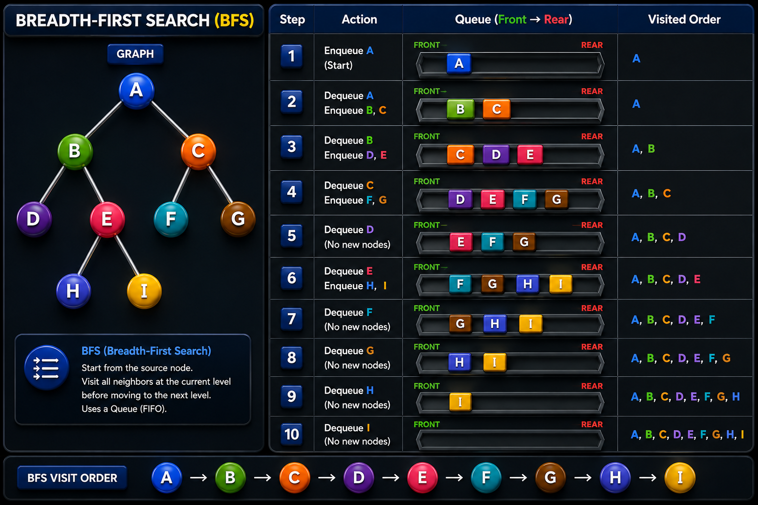
| Step | Queue | Dequeue | Insert | Visited |
|---|---|---|---|---|
| 1 | A | A | B, C | |
| 2 | C B | B | B, C | A |
| 3 | E D C | C | A B | |
| 4 | F E D | D | A B C | |
| 5 | F E | E | A B C D F | |
| 6 | G F | F | A B C D E G | |
| 7 | G | G | A B C D E F | |
| 8 | Empty | Complete |
Let
- = Number of vertices
- = Number of edges
Time Complexity
Each vertex is visited once and each edge is examined at most once.
Space Complexity
The queue and visited set can each store up to all vertices.
Advantages
- Finds the shortest path in an unweighted graph
- Explores vertices level by level
- Guarantees the minimum number of edges to reach a vertex
- Simple to implement using a queue
Disadvantages
- Uses more memory than DFS on wide graphs
- Not ideal for very deep graphs
- Does not work for weighted shortest-path problems
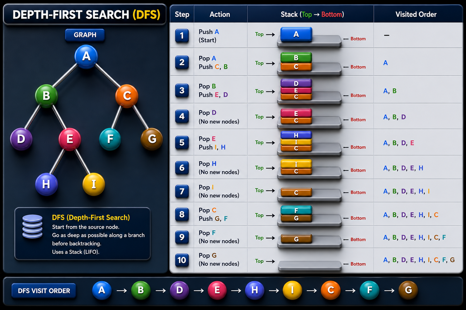
2. Depth-First Search (DFS)
Explores one path as deep as possible before backtracking.
- Uses a Stack (LIFO) or recursion.
DFS Algorithm Steps
- Start from a source vertex.
- Mark it as visited.
- Visit one unvisited neighbor.
- Continue moving deeper.
- If no unvisited neighbors remain, backtrack.
- Repeat until all vertices have been visited.
Backtracking
When a vertex has no unvisited neighbors, DFS returns to the previous vertex.
A
└── B
    └── D
        ↩ Backtrack
        └── E
            └── G
                └── F


A → B → D → E → G → F → C
Complexity
Let
- = Number of vertices
- = Number of edges
Time Complexity
Every vertex and every edge is processed at most once.
Space Complexity
The recursion stack (or explicit stack) and visited set can each contain up to all vertices.
Advantages
- Memory-efficient for deep graphs
- Naturally implemented using recursion
- Excellent for exploring paths
- Useful for recursive problem solving
Disadvantages
- Does not guarantee the shortest path
- Recursive implementation may cause stack overflow on very deep graphs
- Traversal order depends on neighbor ordering
Related Posts
- 🧱 Data Structures — linear structures and the Heap/Hash Table/Trie that round out the non-tree, non-graph structures
- 🌲 Non-Linear Data Structures — trees are graphs with a root and no cycles; see how BST/AVL/Red-Black build on that constraint
- 🔢 Algorithmic Complexity — the Big O notation used throughout this post